1. Introduction

The higher-education system is one of great benefit to enrolledindividuals, the economy, and society, however, an inefficient system with high dropout rates and low throughput rates carries harsh costs and consequences for the individual student as well as the society financing the cost of service delivery [2]. The South African

in the “low economic status civilian” category [3]. Students that belong in this category heavily depend on government study grants and subsidies to supplement the funding they receive from their parents or guardians. It is clear that student debt accumulation, or alternatively, costs to the government without a return on investment will be the outcome when these learners struggle and dropout. This was the case in 2005, where the national treasury reported R4.5 billion lost to student grants and subsidies that resulted in no graduates [3]. There is a student attrition problem in South Africa, as the expansion of enrolments has not come with a significant increase in the percentage of students completing their degrees [4].

Noting the value and possible severe-costs associated with in-

Table 1: This table introduces categories for the different features associated with student performance as discussed in Section 2. The features are divided into four groups, namely, “Socioeconomic Factors” (SEF), “Psycho-Social Factors” (PSF), “Pre & Intra-College Scores” (PICS), and “Individual Attributes” (IA). It is also important to take note of the colour coding scheme developed here for later reference to the four categories, [5](sic).

Family income	Academic self-efficacy	Mathematics	Age at first year
Parents education	Stress and time pressure	English	Work status
Head of house occupation	Class communication	Admission Point Score	Home language
Dwelling value	College activity participation	Accounting	Home province
Dwelling location (rural/urban)	Organization and attention to study	Economic studies	Home country
Financial support	Sense of loneliness	Statistics major	Interest in sports

stitutions of higher-learning, we see the clear need to explore the activities influencing student success or failure to solve the problem of student attrition and avoid the severe costs and consequences that it brings. Furthermore, we seek to develop advanced systems for the early-identification of vulnerable learners that may benefit from academic support systems.

In this research, we investigate the influence of biographical and enrolment observations on student success. This research was conducted through two published studies referred to as “phases of the current study” throughout this paper [5, 6]. In the first phase, we employ six machine learning models to predict three target variables that describe a learner’s end-of-year outcome, namely, “first-year outcome”, “second-year outcome”, and “final outcome” [5]. The first phase of this research contributes to the current body of work by showing that various classification models can be used to predict a learner’s end-of-year outcome from the first year of registration until qualifying in a three-year degree. We argue that if we can predict the academic trajectory of a student, early-assistance can be provided to students who may perform poor in the future, remediating their performance and promoting student success.

The second phase of this study involved the prediction of a “risk profile” variable, a variable that categorises the time taken by a student to graduate in a three-year degree by four values, namely: “no risk”, where the student completes the degree in three years; “low risk”, where the student completes the degree in more than three years; “medium risk”, where the student fails/drops-out in less than three year; and “high risk”, where the student takes more than three years to drop out [6]. We used six machine learning algorithms to predict the “risk profile” variable for a student based on biographical and enrolment observations. The second phase of this study contributes to the current body of related literature in three ways: (1) a comparison of six different classifiers in predicting the risk profile of a learner; (2) a ranking of the features employed according to their contribution when deducing the “risk profile”; and (3) an interactive program which uses Random forests classifier to deduce the distribution over a learner’s risk profile. The contribution made by this research implies institutions of higher-learning can use machine learning techniques for the early-identification of learners that may benefit from academic assistance initiatives.

This paper continues with Section 2 which presents the background knowledge around the problem. We then introduce the procedure and system of methods applied in Section 3, followed by the results in Section 4. The work is concluded on Section 5 and we close this study with ideas of future work in Section 6.

2. Related Work

Predicting student performance is a multifaceted task that cannot be easily completed using attributes discovered in student enrolment records alone [4]. We therefore, set-out to explore the various factors influencing student performance, aiming to discover and develop an efficient methodology for solving the problem set up in this research. We begin this chapter with the discussion and grouping of the factors influencing student performance, followed by a brief presentation of the conceptual framework adopted for feature selection in this research, and we close the chapter with a comparison of the various methods of predicting student performance.

2.1        Factors affecting student performance

The South African Department of Higher Education and Training

(DHET) released a report with results that portray an increasing number of first-time-entering university students, from 98095 students in the year 2000 to over 150000 students in the 2017 academic year [7]. This significant increase brings the idea that the various attributes that describe a university student must be more varied now than ever before, as more learners from different regions are now enrolling for degrees. To accurately early-identify a member of a given group of learners as successful or unsuccessful in their studies, we must explore a wide range attributes that describe these students, so that our decision is informed.

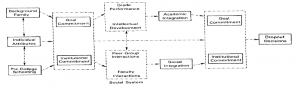
Figure 1: The graphical representation of the framework adopted to determine student success, [6](sic).

2.1.1       Socio-Economic Observations Determining Student Success

To determine an individual or their family’s measure of social and economic position in the population, we explore the category of socio-economic attributes as determinants of student success. Studies have shown that a correlation exists between socio-economic status and academic achievement, furthermore, traditional measures of socio-economic status have been revealed to usually correlate strong enough with academic achievement to account for variations in a learner’s performance [8]. A study of the determinants of student success also concludes that socio-economic factors contribute significantly when predicting a learner’s performance [4]. The socio-economic attributes investigated in the literature we reviewed include; parents’ education, dwelling value, family income, and parent/guardian’s occupation. Family characteristics and financial support also form part of socio-economic factors revealed to explain student performance, specifically drop-out behaviour in university[2].

2.1.2       Psycho-Social Factors Affecting Student Performance

We seek to find more categories of factors that account for variations in a learner’s academic performance. We therefore, explore the combined effects of a student’s thoughts, social factors, and general behaviour at university on academic performance. Research conducted at a South African university found that to predict a learner’s academic performance and adjustment to higher-education, psychosocial factor’s such as; help-seeking attitude, workload, perceived stress, and self-esteem could be utilized as determinants [9].

Research on college students’ performance utilized six psychosocial factors to predict first-year college student success [10]. The six psycho-social attributes used for prediction were; stress and time pressure levels, communication/participation in class, academic self-efficacy (a learner’s belief in their ability to succeed academically), attention to study (measures time-management, planning, and scheduling behaviour), stress levels, and lastly, emotional satisfaction with academics. It was revealed that a strong correlation exists between the six psycho-social factors and a learner’s GPA, these findings align with other related work [11]. A separate study also discovered that academic self-efficacy, student’s optimism, commitment to schooling, and student health account for some of the variations in a student’s performance, expectations and coping perceptions [12].

2.1.3       Factors Available For This Study

The review literature centred around factors affecting student performance revealed that a learner’s mindset, social surrounding, and behaviour, explain significant variations in the performance of a university learner. In this research, student biographical and enrolment observations such as, majors enrolled for, age, pre-college scores, province and country of origin, are available to build machine learning models for the prediction of academic performance. We continue this chapter by introducing the framework we adopted for the rationale behind predicting academic performance from biographical and enrolment observations.

2.2        Conceptual Framework

We use the conceptual framework depicted in Figure 1 as a logical basis to predict the academic performance of a learner from biographical and enrolment observations [13]. The framework develops three categories of attributes contributing to student attrition (dropout behaviour), namely, background attributes, individual attributes, and pre-college scores. The study reveals that these factors together influence a learner’s goal and institutional commitment, which in turn contributes to the drop-out decision of a student via academic and social integration [13]. In this research, we partition background attributes further into socio-economic and psycho-social factors. Table 1 presents the grouping of features discovered to explain variations in academic performance during the review of related literature conducted in this section.

2.3        Methods For Predicting Student Performance

Various authors have already accurately predicted student performance utilizing machine learning. Table 2 compares the accuracies obtained in the various literature reviewed in this research. Acquiring the top accuracy position is a research based on the prediction of the success of a second-year student using an Artificial Neural Network (ANN) model [14]. The study uses individual attributes (IA), pre & intra-college scores, and socio-economic factors as predictors, these inputs are utilized for almost every result presented in the table [11, 17, 16].

3. Research Methodology

This research proposes an approach to the task of university-learnerperformance prediction involving the prediction of a learner’s endof-year outcome from the first year they register for a three-year degree until qualifying to graduate. We complete this task by employing six different machine learning algorithms to deduce the outcomes in the first, second, and final year of study in a South African university. This study extends further by attempting to predict a learner’s risk-profile based on the time it will take the student to complete a three-year degree.

Table 2: The table compares the accuracy achieved by various authors using different machine-learning models to predict academic performance in each case. The table also illustrates for each case, the combination of features used as predictors, based on the feature categories developed in Table 1, [5] (sic).

Author(s)	Factors considered	Model used	Predictive Accuracy
Abu-Naser et al. (2015)[14]	IA, SEF, and PICS	Neural Networks	84.60%
Osmanbegovic and Suljic (2012)[11]	IA, SEF, PICS, and PSF	Naïve Bayes	84.30%
Osmanbegovic and Suljic (2012)[11]	IA, SEF, PICS, and PSF	Neural Networks	80.40%
Osmanbegovic and Suljic (2012)[11]	IA, SEF, PICS, and PSF	Decision Trees (C4.5)	79.60%
Mayilvaganan and Kalpanadevi (2014)[15]	IA and PICS	Decision Trees (C4.5)	74.70%
Ramesh et al. (2013)[16]	IA, SEF, and PICS	Multi-layer Perceptron	72.38%
Abed et al. (2020)[17]	IA, SEF, and PICS	Naïve Bayes	69.18%
Abed et al. (2020)[17]	IA, SEF, and PICS	SMO	68.56%
Ramesh et al. (2013)[16]	IA, SEF, and PICS	Decision Trees (C4.5)	64.88%

In this section, we introduce the procedure and system of methods implemented for the purpose of this study. The study incorporates two phases and thus, we begin by giving a description of the two phases, followed by subsection 3.2 giving a description of the data-sets. We present the feature selection technique in subsection 3.3 and follow this by a brief description of the machine learning models we used, closing the section with methods of evaluating and validating our results.

3.1        Phases of the Study

This study was conducted in two phases. The first phase, named, “Preliminary Phase”, involved generating preliminary results on a synthetic dataset. In this phase we employed six different machine learning models, namely, Decision tree (C4.5), Logistic Model Trees (LMT), Multinomial Logistic Regression, naïve Bayes, Sequential Minimal Optimization (SMO), and Random forests. The purpose of the first phase was to reveal that machine learning models can be utilized for the early prediction of a learner’s end-of-year outcome from the first year of registration until qualifying in a three-year degree, based on biographical and enrolment observations.

The second phase of this study, named, “Post-preliminary Phase”, involved the prediction of the distribution over several risk profiles that describe the time it will take for a university student to complete a three-year degree. This phase is performed on a real dataset which the synthetic dataset in the first phase was modelled to resemble. In this phase we employed six different machine learning models, namely, Decision tree (C4.5), Linear Logistic Regression, Support Vector Machines (SVM), naïve Bayes, and Random forests. This phase provides an interactive program which calculates the posterior probability over a learner’s “risk profile” as the main contribution o this study, and a ranking of features through Information Gain Ranking (IGR), to determine the features most contributing to student performance.

3.2        Data Description and Pre-Processing

Two sets of data were utilized in this study. We therefore, split the description of the datasets, starting with Subsection 3.2.1 which gives the synthetic dataset description, and Subsection 3.2.2 giving a description of the real dataset.

3.2.1       The Synthetic Dataset Description

The dataset used for the preliminary phase of this study is a synthetic dataset generated using Bayesian Network. The dataset was adopted from a recent prediction modelling study aimed at improving student placement at a South African university [17]. In this dataset, conditional independence assumptions were implemented to portray the relationships that exist between enrolment, socioeconomic, and individual attributes found in student records.

Three target variables are investigated in the preliminary phase, namely, “First Year Outcome” (FYO), “Second Year Outcome” (SYO), and “Final Outcome” (FO). The SYO and FYO variables contain two similar possible values: “proceed”, and “failed”, were proceed is the outcome for a student who met the requirements to proceed to the next year of study, and failed implies the student failed to meet the minimum requirements to proceed. The FO variable also has two possible values: “qualified”, and “failed”, were qualified implies the learner met the minimum requirements to graduate in a three-year degree, and failed implies the student failed to meet the requirements to graduate.

Data pre-processing is a crucial step when employing machine learning models. The pre-processing task incorporates, data preparation, data cleaning, data normalization, and data reduction tasks [18]. The synthetic dataset originally contained 50 000 instances. Three random samples (without feature replacement or bias to uniform class) containing 2000 instances were drawn from the raw dataset and several experiments were conducted to make the samples more suitable for our machine learning models. The first set of experiments focused on the detection and removal of outliers or anomalies. This involved the evaluation of classification results from different machine learning classifiers in an attempt to detect and remove instances that display significant deviations from the majority patterns. The second set of experiments conducted aimed to prevent over-fitting. This was done by the implementation of Synthetic Minority Oversampling Technique (SMOTE) which enforced an equal number of training instances for each value in the class variable. The third set of experiments conducted in the preliminary phase is feature selection, where 20 features were selected from each sample based on Information Gain Ranking (IGR) criterion. Subsection 3.3 presents the set of features selected from each sample and a discussion of how we arrived at this set.

3.2.2       The Real Dataset Description

The real data utilized for this study is from a research-intensive university in South Africa. The dataset composes of enrolment and biographical observations of learners enrolled in the faculty of science at the university, from the year 2008 to the year 2018.

The target variable for the post-preliminary phase of this study is “Risk Profile”, a nominal variable that tells us how long it will take for an enrolled student to complete a three-year degree at a South African university. The risk-profile variable has four possible values, namely; “no risk”, where the student completes their degree in 3 years (the minimum allotted time); “low risk”, where the student completes the three-year degree in more than 3 years; “medium risk”, where the student fails to complete the three-year degree before the end of three years (student drops-out in less than 3 years’ time); and “high risk”, where the student fails to complete the three-year degree after exceeding the 3-years period (student drops-out after exceeding the allotted time).

Since our aim is to perform an accurate classification task on the dataset, pre-processing procedures had to be carried out before training the chosen classifiers. We performed the same experiments as those performed on the synthetic dataset to detect and remove outliers. We then employed a sampling procedure similar to the one we implemented in the preliminary phase of this study. Along with applying SMOTE, a random sample (with no replacement of features or bias to uniform class) of 200 instances was drawn from the original dataset. In Subsection 3.3 we present the features selected and the procedure followed to select them.

Table 3: A table providing the various features selected for input into the employed classifiers. The table groups the features according to whether they were used for the prediction of the learner’s first year outcome, second year outcome, or final year outcome. The colour shading gives the category which the feature selected belongs to according to Table 1, [5] (sic).

3.3        Feature Selection

In this subsection we present the methodology behind the features selected for both phases of the study. Subsection 3.2.1 provides the features we utilized to generate the preliminary results and Subsection 3.2.2 provides the features selected for the post-preliminary phase of the study.

3.3.1       Features for the Preliminary Phase

To select features for the purpose of predicting the three target variables investigated in this phase of the study we utilized Information Gain Ranking (IGR) criterion, which involves deducing the contribution of each feature when classifying an instance as a value of the class variable. Table 3 presents the features selected in all cases considered for the preliminary phase, based on the colour coding scheme developed in Table 1.

Feature selection was performed on each of the 3 samples drawn from the synthetic dataset. We investigated the contribution of 44 features using Information Gain (entropy). Through the entropy values and repeated experimentation with different sets of features, a total of 20 features were selected to predict the target variable in each of the three samples.

The features presented in Table 3 are not arranged according to IGR as there are significant differences in the entropy of most features across predicting the three target variables. The features selected align with our findings from the review of previous work, and more importantly, the conceptual framework we adopt in this research [13]. This is because for each target variable, there were features selected from each of the three investigated categories of features, namely, background (socio-economic) attributes, individual attributes, and pre-college scores.

3.3.2       Features for the second phase

To select features for the post-preliminary phase of this study, we continued utilizing IGR alongside the conceptual framework investigated in the related work section [13]. From the “individual attributes” category, the following features were selected; the National Benchmark Test (NBT) scores for academic literacy (NBTAL), quantitative literacy (NBTQL), and mathematical literacy (NBTMA). These scores give a measure of the individual learner’s proficiency and ability to meet the demands of universitylevel work. To further determine an enrolled learner’s professional career aspirations, we also considered the academic plan selected by the learner. The “plan code”, “plan description”, and “streamline” (Earth Science, Physical Science, Biological Science, or Mathematical Science) variables were selected for this task.

From the “background and family” category, the following features were selected; the home-country and province of the student, whether the school attended by the leaner is in the urban or rural areas, the quintile of the school attended, and the age of the learner at the first-year of registration. These variables combined give us a description of the learner’s socio-economic status.

From the pre-college scores category, scores from the following subjects were considered; Mathematics major, Mathematics Literacy, Additional Mathematics, Physical Science, English Home Language, English First Additional Language, Computer studies, and Life Orientation. We note that in this phase of the study, we did not utilize college or university outcomes as inputs, these outcomes were only utilized in the prediction of target variables set up in the preliminary phase as indicated in Table 3. The features selected for the post-preliminary phase of this study are presented ranked according to entropy in Table 6.

3.4        Classification Models

This study composed of two phases, each involving a classification task. In total, we use nine off-the-shelf machine learning predictive models to perform the classification tasks in this research. The models used are: Random forests, naïve Bayes classifier, Decision tree (C4.5), Logistic Model Trees (LMT), Multinomial Logistic Regression, Linear Logistic Regression, Sequential Minimal Optimization (SMO), Support Vector Machines (SVMs), and the K-Star (K*) instance-based classifier. We continue this subsection by giving a brief description of the selected models.

Sequential Minimal Optimization: SMO is an algorithm derived for the improved (speed) training of Support Vector Machines. SVMs previously required that a large quadratic-programming problem be solved in their implementation. Traditional algorithms are slow when training SVMs, however, SMO completes the task much faster by breaking the large quadratic programming problem into a series of smaller problems which are then solved by analytical methods, avoiding the lengthy numerical optimization required. The SMO algorithm we use for the purpose of this study follows the original implementation [19].

Multinomial Logistic Regression: This model derives and extends from the binary logistic regression. It does so by allowing categories of the outcome variable to exceed two. This algorithm utilizes the Maximum Likelihood Estimation (MLE) to predict categorical placement or the probability of category membership on a dependent variable [20]. Multinomial Logistic Regression requires the careful detection and removal of outliers for accurate results, however, the model does not assume or require linearity, homoscedasticity, or normality [20]. An example of a four-category model of this nature, with one independent variable x_i can be given (s)    (s) by:, s = 1,2,3,4. Where; η₀ and η₁ are π_i the slope and intercept respectively, given the probability of cate- (s) gory membership in “s” can be denoted by π_i            , and the selected (0) reference category by π_i . The Multinomial Logistic Regression implementation in this research follows the implementation by other authors before the current study [21, 22].

Naïve Bayes Classifier: The naïve Bayes model is a simplified example of Bayesian Networks. The model achieves learning with ease by assuming that features employed are all independent given the class variable.

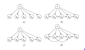
Figure 2: The diagrams (a) to (d) illustrate various examples of a Bayesian network model. The arrows travelling between nodes represent conditional dependencies among the features x₁,x₂,…,x₅,C. Where C, represents the class variable and the models differ based on the existence of a statistical dependence between the predictors (x₁,…,x₅) [18].

The diagram (a) in Figure 2 is an illustration of the naïve Bayes model. This is because the features, x₁,…,x₅ are conditionally independent given the class variable, C. The naïve Bayes independence assumption can be stated as the distribution: P(C|X)=

, where X = (x₁,…,x_n) is a feature vector and C is the class variable. In application, naïve Bayes often performs well when compared to more sophisticated classifiers, although it makes a generally poor assumption [23]. The naïve Bayes model implementation in this research follows other similar implementations in related studies explored; [24, 23].

K* Instance-Based Classifier: The K-Star algorithm classifies instances using training instances that are similar to them alongside a distance function that is based on entropy. The use of an entropy based function provides consistency in the classification of instances in our experiments that may be real-valued or symbolic.The K* implementation utilized for the purpose of this research followed the implementation by [25].

Support Vector Machines:The (SVMs) classification model separates classes of the training data with a hyper-plane. The test instances then get mapped on the same space with their prediction based on the side of the hyper-plane they belong after splitting. This task is performed by incorporating the training dataset into a binary linear classifier that is non-probabilistic. SVMs can be scaled through the one-versus-all partitioning, for various types of classification problems including high-dimensional and nonlinear classification tasks. The SVM model implementation in this research follows the implementation in other related work [26].

Linear Logistic Regression: The Linear Logistic Regression model utilizes additive logistic regression with simple regression functions as base learners of the algorithm [27].The implementation of this model followed in this research follows that of related work conducted in the past [28, 29].

Decision Tree: This model uses a decision support system to build a classification function that predicts the value of a dependent variable given the values of independent variables, through tree-like graph decisions and their possible after-effect, including costs of resources, chance results, and utility [30]. There are different algorithms for generating decision trees; C4.5, Random forest, and LMT are the tree-models selected for the purpose of this research.

The C4.5 algorithm uses information gain to build a decision tree, selecting features based on entropy and utilizing the ID3 algorithm recursively to build the tree. We follow the original structure and implementation of the C4.5 algorithm in this study [31].

LMT builds a single tree from a combination of logistic regression models and a tree structure. This model accomplishes the combination by using the Classification and Regression Tree (CART) algorithm to prune after building the regression functions through the LogiBoost algorithm. The LMT method used in this study follows from the original implementation [28].

Random Forests are a combination of decision tree predictors dependent on the value of a random vector, where the value also governs the growth of each tree in the generated forest. This algorithm involves utilizing the training data to generate an ensemble of decision trees and allowing them to decide on the most-popular class. Implementing this technique has several advantages, including that, the procedure abides by the Law of Large Numbers to prevent over-fitting, it is relatively robust to noise or outliers in data, and the model achieves accuracy as good as similar techniques such as, Adaboost, Bagging, and Boosting, while still training faster than them [32]. The Random forest model implementation in this research is based on the original model [32].

3.5        Prediction and Evaluation

In this research, the dataset contains the dependent attribute and the values of the classes are known, we therefore have a classification task set up. This subsection provides the measures and techniques utilized to complete this task.

3.5.1       Evaluation and Validation

10-fold cross-validation procedure is applied to evaluate each model employed in this research. In this validation procedure, the training dataset is partitioned such that a portion (testing data) of it is not provided to the algorithm during training, but is used for the validation. The partition remaining for training is further split into 10 partitions (folds). Interchangeably, each of the 10-folds serve for validation while the remaining 9 are used for training until all 10-folds serve as the validation fold once.

3.5.2       Confusion Matrix

We use confusion matrices to illustrate classification outcomes. Table 4 provides an example of the format of a confusion matrix.

Table 4: This table depicts the structure of a confusion matrix. We denote “negative” and “positive” by -ve & +ve respectively. Where TP are the true positives (correctly classified positives), FP the false positives, FN are false negatives, and TN are the true negatives (correctly classified negatives).

	Predicted Class +ve	Predicted Class -ve
Actual Class +ve	TP	FP

3.5.3       Accuracy

We extract precision and recall metrics from the confusion matrix in order to measure the accuracy of the employed machine learning models. “Precision” represents the correctly real-positive proportion of predicted positives, while “Recall” represents the correctly predicted proportion of the real positives. We calculate precision and recall as follows:

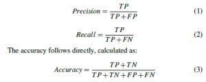
This representation of accuracy has been used in other related work [17], [33]. Other measures of accuracy explored include the Receiver Operating Characteristic (ROC) curve. This curve plots recall (the true positive rate) against the false positive rate (ratio between FP and the total number of negatives), and the area under the ROC reflects the probability that prediction is informed versus chance [34]. We desire the ROC-area to lie above 0.5, anything below 0.5 implies the prediction was guesswork and not informed. Another accuracy measure utilized is the F-beta measure (F1 score), which calculates a test accuracy as the weighted harmonic mean of precision and recall. The optimal value for the F-measure is 1 (indicating perfect precision and recall), and the worst value is 0.

4. Results and Discussion

This study was conducted in two phases. The first phase involved generating preliminary results on a synthetic data-set, while in the second phase, a similar set of experiments are performed on a real data-set, leading to conclusions and implications about the performance of the trained machine learning models in classifying the problem at hand, furthermore, the results drawn from the second phase provide a ranking of the employed features according to entropy, together with an interactive program which calculates the posterior probability over the students’ risk profile so that support initiatives and programs can be focused on them.

4.1        Preliminary Results

This Subsection presents the results of six of the nine prediction models discussed in Section 3, namely; Decision tree (C4.5), Logistic Model Trees (LMT), naïve Bayes Classifier, Sequential Minimal Optimization (SMO), Multinomial Logistic Regression, and Random Forests. We present first the prediction outcomes through a table comparing predictive accuracy of the models as determined by Equation 3. This will be followed by an evaluation of the model’s performance through F-measure and Receiver Operating Characteristic (ROC) curve.

4.1.1       Prediction Outcomes

Six different machine learning models were utilized to solve our classification problem. The predictive accuracy achieved by each model is recorded and presented in the Table 5.

Table 5: Predictive accuracy as calculated by Equation 3. After 10-fold crossvalidation, all of the models utilized achieved an accuracy above 80%, with Random Forests achieving top accuracy in all three cases considered, [5](sic).

Predictive Accuracy

    Model used                           1^st Year Outcome           2^nd Year Outcome          Final Year Outcome

Random Forest	94.40%	93.70%	95.45%
LMT	91.90%	91.75%	93.15%
Decision Trees (J48)	87.55%	86.20%	91.45%
Multinomial Logistic	87.80%	86.20%	90.70%
SMO	87.25%	84.45%	89.20%
Naïve Bayes	83.95%	83.40%	84.40%

4.1.2       Model Performance Evaluation

A study based on evaluating classification results argued for the use of Precision, Recall, F-Measure, and the ROC curve, as accurate measures of a machine learning model performance [34]. We utilize these measures to evaluate results presented by Figure 3, 4, and 5.

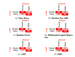
Figure 3: The set of confusion matrices resulting from the prediction of first-year outcome. Evaluation of the accuracy by class reveals that the weighted average of both precision and recall lies above 0.84 for all six models trained in our study. Further observations reveal that the f-measure of accuracy is more than 0.83 for all models, this value aligns with our accuracy as determined by Equation 3 in the Table 5. The test accuracy obtained in the table is further supported by the ROC curve obtained for all six models, as the weighted average of the ROC area for each model is more than 0.84 implying the models trained were making informed decisions in classifying the problem and not simply guessing.

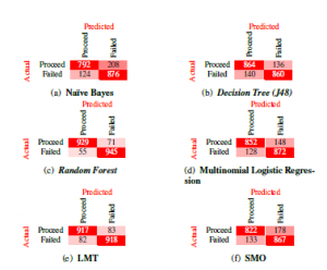
Figure 4: The confusion matrices obtained when classifying the second-year outcome variable. When we evaluate the detailed accuracy by class for each model, we find that the weighted average of both precision and recall measures is above 0.83, furthermore, the f-measure of test accuracy aligns with our findings in Table 5 with a value of more than 0.83 for all six models considered. The ROC curve obtained for all six models also aligns with our accuracy as determined by f-measure of test accuracy and Equation 3, as the weighted average of the area under the ROC curve lies above 0.85 implying the models trained are not attaining the great predictive accuracy through guess-work, but they are making informed predictions.

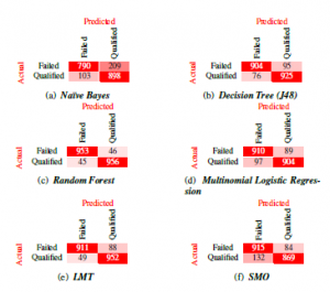
Figure 5: Confusion matrices obtained when classifying the third-year outcome variable with the six trained machine learning models. Evaluating the detailed accuracy by class results, we find that the weighted average of both precision and recall measures is more than 0.89 for all models except the naïve Bayes classifier which scored 0.85 for precision, and 0.84 for recall. The underperformance of the naïve Bayes model with respect to other trained classifiers can be explained by the naïve feature-independence assumption it makes. Results also show that the weighted average of the area under the ROC curve for each model is in alignment with our test accuracy measures, as it lies above 0.89, implying each model is making informed predications and not simply guessing the outcome.

4.2        Main Results (Post-preliminary)

The preliminary phase of this study revealed that we can utilize machine-learning models to accurately predict a learner’s outcome from the first year of registration until qualifying in a three-year degree. The preliminary results confirmed our initial hypothesis but furthermore, revealed the kind of model we should utilize with such a wide variety of models available for use, but few fitted to the problem set up in this study. Evaluating the preliminary results, we note that Random Forests achieved top accuracy and performance as measured by all our model performance and accuracy evaluators, across all three test cases.

In this subsection, we present the results obtained when utilizing machine learning models to classify a learner into the four risk profiles (“No Risk”, “Low Risk”, “Medium Risk”, and “High Risk”) defined in Section 3, as the preliminary phase has confirmed this task can be completed. The classification problem set up in this phase is parallel to that in the prelim-phase in several ways, as the preliminary phase utilizes a synthetic data-set modelled to resemble the relationships that exist within the student enrolment data utilized for the second phase.

Subsection 4.2.1 presents the selection and ranking of features utilized, we follow this by a presentation of the classification outcomes and close the section with the presentation of an interactive program that can be utilized to calculate the posterior probability over a student’s risk profile.

4.2.1       Selection and Ranking of features

We selected 20 features to predict the class variable. The features were selected using Information Gain Ranking (IGR) to deduce the contribution of each feature in classifying the instances. The feature selection findings are illustrated through Table 6 with three columns below. The first column determines the rank of the features among the input set, the second column gives the amount of entropy attained by the feature, and the third column has the name of the feature associated with the ranking and entropy.

Table 6: A ranking through information gain (entropy) of the set of features selected to predict the student risk profile, ranked from the most contributing feature to the least contributing feature. The top seven features that are highlighted indicate an entropy greater than 0.1, [6] (sic).

       Rank       Entropy            Feature Name

1			1.21960228	PlanCode
2			1.15086266	PlanDescription
3			0.59886383	Streamline
4			0.29582771	Year Started
5			0.20836689	AgeatFirstYear
6			0.18695721	SchoolQuintile
7			0.14234042	MathematicsMatricMajor
	8	0.12166049			Homeprovince
	9	0.06417526			isRuralorUrban
	10	0.0568866			LifeOrientation
	11	0.04978826			PhysicsChem
	12	0.02780914			EnglishFirstLang
	13	0.01253064			Homecountry
	14	0.00550434			AdditionalMathematics
	15	0.00000902			MathematicsMatricLit
	16	< 0.00001			NBTAL
	17	< 0.00001			NBTMA
	18	< 0.00001			NBTQL
	19	< 0.00001			ComputerStudies
	20	< 0.00001			EnglishFirstAdditional

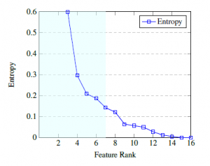
Figure 6: A graphical illustration of how the information gain (entropy) level varies across the chosen feature input set. The x-axis indicates the feature rank, and the y-axis indicates the information gain from utilizing the corresponding feature, [6] (sic).

The use of IGR also has implications on the contribution made by a feature relative to others within the chosen input set of features. We investigate the behavior of entropy as you move between subsequent features and present the findings through a graphical illustration in Figure 6, showing the monotonically decreasing behavior of the entropy function plotted versus rank. We see that the loss in entropy between each subsequent point (feature rank) is logarithmically decreasing, furthermore, we highlight the same top seven features from the IGR Table 6.

The highlighted features on Figure 6 illustrates their relative importance in forecasting the success of a learner. We note that the set of factors most contributing to a learner’s success includes, “the plan-code and plan description” (combined, these two variables give a precise description of what the student is studying), “streamline” (mathematical, life, or physical science), “the year started”, “school quantile”, “age at first-year”, and “the student’s matric mathematics score”.

4.2.2       Classification Outcomes

This section presents the results obtained from the classification algorithms trained to predict the class variable (risk profile). Six of the nine classification procedures discussed in Section 3 were employed for the post-preliminary phase of the study: Decision trees (C4.5), naïve Bayes Classifier, Linear Logistic Regression model, Support Vector Machines (SVMs), K*, and Random Forests.

Figure 7 (a) – (f) illustrates the results of each trained classifier after 10-fold cross-validation. Evaluating the performance of each model relative to other models employed, we note that the Random forests classifier attains the highest accuracy (83%) of all the models trained for the post-preliminary phase. This result aligns with our findings from the preliminary phase of the study as Random forests attained the highest accuracy among the selected models for both phases of the study.

We note further that the SVM classification model was revealed to be the least suited for the problem set up in this study. At 52%, SVMs attained the lowest predictive accuracy in this study, furthermore, SVMs took the longest time to train. When discussing training and testing times, it is also important to note that the K-star model took the least time to implement in this study.

Overall, the classification task was a success, with five of the six models employed attaining a predictive accuracy above 75%. Noting that Random forests was the most accurate in predicting the class variable for both phases of this study, this section continues by providing a web application utilizing the Random forests classifier to predict the risk-profile of a learner based on enrolment and academic factors. Severity of misclassified instances was also evaluated and taken into account to determine Random forests as the most suited model for the task, for example, the 27% of “No Risk” instances incorrectly classified by SVM as “Medium Risk” is far more severe and misleading than the misclassification of 5% “No Risk” instances as “Medium Risk” by Random forests classifier.

4.2.3       Main Contribution of The Study

In this subsection we provide an interactive program which can calculate the posterior probability over a student’s risk profile utilizing the Random forests model employed in Section 4.2.2. This automated system makes predictions about a student’s risk of failure based on the conceptual framework developed in a “drop-out from higher education” study [13]. The conceptual framework connects dropout decision to categories of input features, namely, background (family) attributes, individual attributes, and pre-college scores. This framework is better depicted in the Figure 1 provided under the related work section.

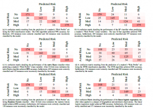
Figure 7: A set of confusion matrices obtained when classifying the “Risk Profile” variable. We provide the accuracy of each classification model as determined by Equation (*****) along with a count of the correctly and incorrectly classified instances by each model, [6] (sic).

The web application depicted in Figure 8 provides a practical tool which university student support programs can utilize for early detection of learners in need of academic support. We argue that the early detection and assistance of students at risk of failure is likely to lead to improved academic performance and eventually higher pass-rates, which translate to increased throughput rates.

The example depicted in Figure 8 illustrates the calculation of the risk profile of a learner based on biographical and enrolment observation. The program predicts the posterior distribution over the four “Risk Profiles”, namely, “No Risk”, “Medium Risk”, “High Risk”, and “Low Risk” using the Random forests classifier. The learner in the example is from an urban quantile 3 school in Kwazulu-Natal South Africa, furthermore, individual attributes are provided as follows; scores of 48%, 50%, and 55% for the quantitative, academic, and mathematical literacy National-BenchmarkTests (NBT) respectively. The learner also completed pre-college courses with scores of; 50% for both core Mathematics and Life Orientation, and 60% for English Home Language. The output presented at the bottom of Figure 8 illustrates that hypothetically the student is 10% likely to complete their degree in 3 years (No Risk), 50% likely to complete their degree in greater than 3 years (Low Risk), 35% likely to drop-out before the end of 3 years (Medium Risk), and 5% likely to drop-out in greater than 3 year (High Risk). With the output obtained, students support-program-coordinators can then decide what assistance will prove most beneficial to the student in the example as the learner posses a high chance of struggling to complete their degree in the allocated time (50% Low Risk).

5. Implications and Conclusions

The expansion of enrolments in South African universities has not been accompanied by a proportional increase in the percentage of learners graduating. In this study, we took on the task of early prediction of a learner’s academic trajectory, aiming at identifying those who may struggle in universities, so that proactive learner remediation to promote success may be provided to them.

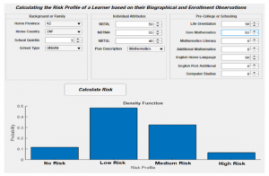
Figure 8: The graphical user interface for the at-risk program, [6](sic).

This paper contributes to the current body of knowledge firstly by introducing an approach involving the prediction of a learner’s outcome from the first year of registration until qualifying in a threeyear degree. We argue for the early prediction of a learner’s entire academic trajectory with the aim to detect those who are likely to benefit from student academic support initiatives. We trained six machine learning models to predict first, second, and final year outcomes from a synthetic data-set. After 10-fold cross-validation this task was completed with great success as all six models attained an accuracy above 83%. Furthermore, an evaluation of the F-measure of accuracy and ROC-curve reveal that these models are making informed-accurate decisions and not simply guessing, therefore, leading to our second contribution involving a real data-set from a research-intensive university in South Africa.

The second contribution of this study is a ranking (through entropy) of features according to their contribution in correctly predicting a learner’s “risk profile” (class variable). The ranking of features according to entropy reveals which features are stronger determinants of student success relative to others employed and, in this study, we highlight the seven top-ranked features, namely, “plan code”, “plan description”, “year started”, “age at first year”, “streamline”, “school quantile”, and “Matric Mathematics major”.

The third and main contribution made by this study is an interactive program which can predict the distribution over a learner’s risk profile utilizing biographical and enrolment observations. The interactive program proposed in this paper can be utilized for early identification of university learners who are most likely to benefit from student support initiatives aimed at improving academic performance. The implication of this study is that university learners can be assisted early in their academic journey increasing their chances of success. Furthermore, the early detection and assistance of learners in need of academic support will result in an improved and enriched learning experience beyond what the student would have experienced if support initiatives were implemented after failure has been detected.

6. Future work

To continue with the work done in this paper, future work may involve: (a) incorporating into our models features from categories not considered such as the “psycho-social attributes category”, (b) exploring what courses offered in university possess high failure rates and how good the set of features we employed predict success in these courses, or (c) approaching the problem from a different perspective by attempting to predict which courses are students likely to struggle completing so that support initiatives may be focused on the specific courses.

Conflict of Interest

The authors declare no conflict of interest.

Acknowledgement

This work is based on the research supported in part by the National Research Foundation of South Africa (Grant number: 121835).

1. J. V. Winters, “Human capital, higher education institutions, and quality of life,” Regional Science and Urban Economics, 41(5), 446–454, 2011, doi: 10.1016/j.regsciurbeco.2011.03.001.
2. G. Lassibille, L. N. Gómez, “Why do higher education students drop out? Evidence from Spain,” Education Economics, 16(1), 89–105, 2008, doi: 10.1080/09645290701523267.
3. M. Letseka, S. Maile, High university drop-out rates: A threat to South Africa’s future, Human Sciences Research Council Pretoria, 2008.
4. K. G. Bokana, D. D. Tewari, “Determinants of Student Success at a South African University: An Econometric Analysis,” The Anthropologist, 17(1), 259–277, 2014, doi:10.1080/09720073.2014.11891436.
5. N. Ndou, R. Ajoodha, A. Jadhav, “A Case Study: Educational Data-mining to Determine Student Success at Higher Education Institutions,” in The Interna- tional Multidisciplinary Information Technology and Engineering Conference, 2020.
6. R. Ajoodha, A. Jadhav, S. Dukhan, “Forecasting Learner Attrition for Student Success at a South African University,” in Conference of the South African Institute of Computer Scientists and Information Technologists 2020 (SAICSIT ’20), September 14-16, 2020, Cape Town, South Africa. ACM, New York, NY, USA, 10 pages., ACM, 2020, doi:10.1145/3410886.3410973.
7. D. H. E. T. Department of Higher Education & Training Republic of South Africa, “2000 to 2017 first time entering undergraduate cohort stud- ies for public higher education institutions,” Annual report, 16–28, 2020.
8. K. R. White, “The relation between socioeconomic status and academic achievement.” Psychological Bulletin, 91(3), 461–481, 1982, doi:10.1037/ 0033-2909.91.3.461.
9. M. Sommer, K. Dumont, “Psychosocial Factors Predicting Academic Per- formance of Students at a Historically Disadvantaged University,” South African Journal of Psychology, 41(3), 386–395, 2011, doi:10.1177/ 008124631104100312.
10. E. J. Krumrei-Mancuso, F. B. Newton, E. Kim, D. Wilcox, “Psychosocial Factors Predicting First-Year College Student Success,” Journal of College Student Development, 54(3), 247–266, 2013, doi:10.1353/csd.2013.0034.
11. E. Osmanbegovic, M. Suljic, “Data mining approach for predicting student performance,” Economic Review: Journal of Economics and Business, 10(1), 3–12, 2012.
12. M. M. Chemers, L. Hu, B. F. Garcia, “Academic self-efficacy and first year col- lege student performance and adjustment.” Journal of Educational Psychology, 93(1), 55–64, 2001, doi:10.1037/0022-0663.93.1.55.
13. V. Tinto, “Drop-Outs From Higher Education: A Theoretical Synthesis of Recent Research,” Review of Educational Research, 45, 89–125, 1975, doi: 10.2307/1170024.
14. S. A. Naser, I. Zaqout, M. A. Ghosh, R. Atallah, E. Alajrami, “Predicting Stu- dent Performance Using Artificial Neural Network: in the Faculty of Engineer- ing and Information Technology,” International Journal of Hybrid Information Technology, 8(2), 221–228, 2015, doi:10.14257/ijhit.2015.8.2.20.
15. M. Mayilvaganan, D. Kalpanadevi, “Comparison of classification techniques for predicting the performance of students academic environment,” in 2014 International Conference on Communication and Network Technologies, IEEE,
    2014, doi:10.1109/cnt.2014.7062736.
16. V. Ramesh, P. Parkavi, K. Ramar, “Predicting Student Performance: A Statisti- cal and Data Mining Approach,” International Journal of Computer Applica- tions, 63(8), 35–39, 2013, doi:10.5120/10489-5242.
17. T. Abed, R. Ajoodha, A. Jadhav, “A Prediction Model to Improve Student Placement at a South African Higher Education Institution,” in 2020 Inter- national SAUPEC/RobMech/PRASA Conference, IEEE, 2020, doi:10.1109/ saupec/robmech/prasa48453.2020.9041147.
18. S. García, J. Luengo, F. Herrera, Data preprocessing in data mining, Springer, 2015.
19. J. Platt, “Sequential Minimal Optimization: A Fast Algorithm for Training Support Vector Machines,” Technical Report MSR-TR-98-14, 1998.
20. D. Böhning, “Multinomial logistic regression algorithm,” Annals of the Institute of Statistical Mathematics, 44(1), 197–200, 1992, doi:10.1007/ bf00048682.
21. B. Krishnapuram, L. Carin, M. Figueiredo, A. Hartemink, “Sparse multinomial logistic regression: fast algorithms and generalization bounds,” IEEE Trans- actions on Pattern Analysis and Machine Intelligence, 27(6), 957–968, 2005, doi:10.1109/tpami.2005.127.
22. Y. Wang, “A multinomial logistic regression modeling approach for anomaly intrusion detection,” Computers & Security, 24(8), 662–674, 2005, doi: 10.1016/j.cose.2005.05.003.
23. I. Rish, et al., “An empirical study of the naive Bayes classifier,” in IJCAI 2001 workshop on empirical methods in artificial intelligence, volume 3, 41–46, 2001.
24. R. Ajoodha, Influence Modelling and Learning Between Dynamic Bayesian Networks Using Score-based Structure Learning, University of the Witwater- srand, Faculty of Science, School of Computer Science and Applied Mathe- matics, 2018.
25. J. G. Cleary, L. E. Trigg, “K*: An Instance-based Learner Using an Entropic Distance Measure,” in 12th International Conference on Machine Learning, 108–114, 1995, doi:10.1016/b978-1-55860-377-6.50022-0.
26. C.-C. Chang, C.-J. Lin, “LIBSVM,” ACM Transactions on Intelligent Systems and Technology, 2(3), 1–27, 2011, doi:10.1145/1961189.1961199.
27. J. Friedman, T. Hastie, R. Tibshirani, “Additive Logistic Regression: A Sta- tistical View of Boosting,” The Annals of Statistics, 28, 337–407, 2000, doi: 10.1214/aos/1016218223.
28. N. Landwehr, M. Hall, E. Frank, “Logistic Model Trees,” Machine Learning, 59, 161–205, 2005, doi:10.1007/s10994-005-0466-3.
29. M. Sumner, E. Frank, M. Hall, “Speeding up Logistic Model Tree Induc- tion,” in 9th European Conference on Principles and Practice of Knowledge Discovery in Databases, 675–683, Springer Berlin Heidelberg, 2005, doi: 10.1007/11564126_72.
30. M. J. Zaki, W. Meira, Jr, Data Mining and Analysis: Fundamental Con- cepts and Algorithms, Cambridge University Press, 2014, doi:10.1017/ CBO9780511810114.
31. J. Quinlan, C4.5: Programs for Machine Learning, Ebrary online, Elsevier Science, 2014.
32. Y. L. Pavlov, Random Forests, De Gruyter, 2000, doi:10.1515/9783110941975.
33. S. Sahu, B. M. Mehtre, “Network intrusion detection system using J48 De- cision Tree,” in 2015 International Conference on Advances in Computing, Communications and Informatics (ICACCI), IEEE, 2015, doi:10.1109/icacci. 2015.7275914.
34. D. M. W. Powers, “Evaluation: from precision, recall and F-measure to ROC, informedness, markedness and correlation,” 2020.

(Click Here)

(Click Here)