
Towards a Hybrid Probabilistic Timing Analysis
Volume 6, Issue 1, Page No 1360-1368, 2021
Author’s Name: Haoxuan Li1,a), Ken Vanherpen2, Peter Hellinckx3, Siegfried Mercelis3, Paul De Meulenaere2
View Affiliations
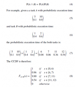
1Faculty of Applied Engineering, CoSys-Lab, University of Antwerp, Antwerp, 2000, Belgium
2Faculty of Applied Engineering, CoSys-Lab, University of Antwerp – Flanders Make, Antwerp, 2000, Belgium
3Faculty of Applied Engineering, IDLab, University of Antwerp – imec, Antwerp, 2000, Belgium
a)Author to whom correspondence should be addressed. E-mail: Haoxuan.Li@uantwerpen.be
Adv. Sci. Technol. Eng. Syst. J. 6(1), 1360-1368 (2021); ![]() DOI: 10.25046/aj0601155
DOI: 10.25046/aj0601155
Keywords: Hybrid Timing Analysis, Worst-Case Execution Time, Probabilistic Timing Analysis, Real-Time Systems, Hybrid Probabilistic Timing, Analysis

Export Citations
Real-time embedded systems are widely adopted in applications such as automotive, avionics, and medical care. As some of these systems have to provide a guaranteed worst-case execution time to satisfy the time constraints, understanding the timing behaviour of such systems is of the utmost importance regarding the reliability and the safety of these systems. In the past years, various timing analysis techniques have been developed. Probabilistic timing analysis has recently emerged as a viable alternative to state-of-the-art deterministic timing analysis techniques. Since a certain degree of deadline miss is still tolerable for some systems, instead of deriving an estimated worst-case execution time that is presented as a deterministic value, probabilistic timing analysis considers execution times as random variables and associates each possible execution time with a probability of occurrence. However, in order to apply probabilistic timing analysis, the measured execution times must be independent and identically distributed. In the particular case of hybrid timing analysis, since the input and the initial processor state of one software component are influenced by the preceding components, it is difficult to meet such prerequisite. In this article, we propose a hybrid probabilistic timing analysis method that is able to (i) reduce the dependence in the measured execution times to facilitate the application of extreme value theory and (ii) reduce the dependence between software components to make it possible to use convolution to calculate the probabilistic WCET of the overall system.
Received: 21 December 2020, Accepted: 09 February 2021, Published Online: 28 February 2021
1. Introduction
Due to the demand for better performance and the increased number of functionalities in embedded systems, acceleration features, such as multi-cores and caches, are added to the modern processors [1]. However, because of these acceleration features, timing analysis has become more complicated and time-consuming.
Over the past years, various researches have been carried out to develop timing analysis techniques that can derive a sound and safe result within a reasonable cost. With “sound”, it is meant that a timing analysis result is accurate and not overly optimistic concerning its timing behaviour. The word “cost” describes the time and effort spent on deriving a timing analysis result. In the plethora of techniques, probabilistic timing analysis (PTA) has recently emerged as a viable alternative to state-of-the-art deterministic timing analysis techniques.
In real-time systems, failing to meet the deadline does not necessarily imply a failure of the system. For instance, in video confertiming requirement does not always have to be strictly guaranteed, and a certain degree of deadline misses is still tolerable. Therefore, Instead of deriving an estimated worst-case execution time (WCET) that is presented as a deterministic value, PTA considers execution times as random variables and associates each possible execution time with a probability of occurrence.
Figure 1 is the examples of the probabilistic WCET (pWCET) and the deterministic WCET, as well as the terminologies we use through this paper. The authors suggested that since the upper timing bound derived using the probabilistic worst-case execution time (pWCET) can be adjusted according to the safety requirement of the system, probabilistic timing analysis (PTA) is supposed to be more flexible and potentially less pessimistic compared with the classical deterministic approaches [2]. Therefore, we developed our approach based on the work in [3, 4] with measurement-based probabilistic timing analysis (MBPTA).
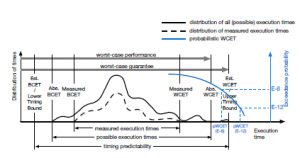
Figure 1: Examples of pWCET analysis and deterministic WCET timing analysis (based on [5]).
One prerequisite of applying MBPTA is that the measured execution times must be independent and identically distributed (i.i.d.). However, in hybrid timing analysis, the input and the initial processor state of one code block/component are influenced by the preceding code/component. Therefore, it is very challenging to collect execution times following the independent and identical distribution.
In this article, we present a hybrid probabilistic timing analysis (HPTA) approach that can facilitate in conducting MBPTA on software blocks/components and safely construct the overall execution of the complete program by reducing the dependence in the measured execution times and the dependence between the components. The goal of this approach is to provide more flexibility in the timing analysis results, which can be used by experienced engineers as references when designing non safety-critical systems that can tolerate a certain degree of deadline misses.
The rest of this paper is organised as follows. Section 2 gives the background of PTA. Section 3 explains the details of the extreme value theory (EVT) and how to apply it in MBPTA and HPTA. The proposed HPTA method is presented in Section 4. Section 5 demonstrates the experiment setup and the case studies, followed by the results and discussion in Section 6.
2. Background
The acceleration features of the hardware, the different input values, and the paths taken through the software introduce a certain degree of variability to the execution time of a system [6]. Because of such variability, PTA considers each observed execution time as an event with a probability of occurrence. Thus the worst-case execution time (WCET) can be viewed as an event that is more extreme than any previously observed event [7].
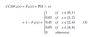
PTA derives a cumulative distribution function (CDF) using the observed execution times in the measurement. Since PTA aims to provide the probability that one execution time is going to exceed a given time bound, the result is usually presented as a complementary cumulative distribution function (CCDF) [8, 9, 10].
Figure 2 is an example of the results in measurement-based probabilistic timing analysis (MBPTA). The EVT takes the measured execution times to generate the CCDF. This CCDF-function then represents the probability that an event will have an execution time larger than a given pWCET value. This way, every pWCET is associated with such an exceedance probability. For example, in the given figure, the pWCET shows that for every execution of the program, the probability of the execution time exceeding 9.6ms is 1E-16.

Figure 2: Example of the analysis result of one MBPTA shown as CCDF [11].
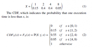
For instance, to calculate the pWCET of a task with the probability that the execution time will be 1 time unit is 0.15, the probability that the execution time will be 2 is 0.4, the probability that the execution time will be 4 is 0.4 and the probability that the execution time will be 8 is 0.05. The discrete probability distribution function of execution times of this task can be expressed in the form of a probability mass function (PMF), which is also known as execution time profile (ETP) in the context of PTA:
Eventually, the CCDF is generated to represent the analysis results because pWCET analysis rather focuses on the probability that an execution time exceeds a particular level:
CCDFX(x) = F¯X(x) = P(X > x)
3. Extreme Value Theory
EVT is a branch of statistics that is used to assess the probability of the occurrence of rare events based on previous observations [8]. It has been widely applied in many disciplines such as finance, earth sciences, traffic prediction, and geological engineering. In MBPTA, EVT is used to analyse the tail behaviour of the execution time distribution based on the execution times observed during the measurement.
3.1 Independent and identical distribution
The prerequisite of EVT requires the observations to be independent and identically. Independent means that the occurrence of one event does not impact the occurrence of the other event. Identical indicates that each measured execution time is random and has the same probability distribution as the others.
In the context of timing analysis, i.i.d. implies that the measured execution time is not affected by the past events of the same task. For example, task A is executed twice consecutively on a processor with a first-in-first-out (FIFO) cache. The measured execution time is x for the first time and y for the second time. Because the cache is loaded with data and instructions needed after the first time the task is executed, y is expected to be much smaller compared with
- x. In this case, the execution time x and y are said to be dependent,
which does not meet the i.i.d. requirement.
Previous research has proposed the adoption of randomised architectures for measurement-based probabilistic timing analysis[12, 13]. If the processor of the target system has a deterministic architecture, randomisation needs to be applied to randomise the measurement samples to satisfy the i.i.d. precondition [9, 14, 15].
If two events are independent, the joint probability is equal to the product of their individual probabilities:
3.2 Applying extreme value theory in measurementbased probabilistic timing analysis
Algorithm 1 demonstrates how to apply EVT in MBPTA, which includes three main steps: (1) extreme value selection; (2) fitting the distribution; (3) compare and convergence.
Algorithm 1: How to apply EVT in MBPTA
Result: pWCET
select extreme values;
3.2.1 Extreme value selection
EVT makes assumptions on the tail of the data distribution based on the extreme observations obtained from the measured data. Therefore, the measured execution times of the program must be converted into a set of extremes before applying the EVT. Two approaches can be used to collect the observed extreme execution times: block maxima (BM) and peak over threshold (POT).
The BM approach divides the collected execution times into subgroups/blocks. The longest execution time in every subgroup is one sample of extremes. The POT approach defines a threshold. All the execution times longer than the threshold are used as the extremes to estimate the pWCET.
The selection of a suitable size of the subgroups in the BM or a suitable threshold value in the POT plays a crucial role. Studies have been carried out to determine the impact of these decisions on the estimated results [2, 16, 17]. Neither an optimal size of the subgroups nor the best threshold value exists. Generally speaking, a smaller subgroup size or a lower threshold value can decrease the pessimism in the results. However the risk of obtaining an overly optimistic pWCET that is not safe to use increases.
3.2.2 Fitting the distribution
In this step, a model distribution that best fits the extremes is estimated. If BM was used in the previous step, the distribution must be Gumbel, Frechet, or Weibull distribution. These three distributions´ are combined into a family of continuous probability distributions known as the generalised extreme value (GEV) distribution.
The GEV is characterised by three parameters: the location parameter µ ∈R, the scale parameter σ > 0, and the shape parameter ξ ∈R. The value of the shape parameter ξ decides the tail behaviour of the distribution and to which sub-family the distribution belongs: Gumbel (ξ = 0), Frechet (´ ξ > 0) or Weibull (ξ < 0). The CDFs of these three distributions are given below.
- Gumbel or type I extreme value distribution (ξ = 0):
- Frechet or type II extreme value distribution (´ ξ > 0):
- Reversed Weibull or type III extreme value distribution (ξ < 0):
If POT was used in the previous step, the distribution needs to fit the generalised Pareto distribution (GPD), which is a family of continuous probability distributions. The GPD is specified by the same three parameters as GEV: location parameter µ , scale parameter σ , and shape parameter ξ. The CDF of the GPD is:
3.2.3 Compare and convergence
Once the first data set of extremities is collected, the EVT uses the data to estimate the first CDF of the pWCET. In every subsequent round of the estimation, more extremities are collected and added to the data set to derive a new CDF. The CDF in the current round is compared with the CDF of the previous round using metrics such as the continuous ranked probability score (CRPS) [18]. In our case, we use the following convergence criteria to compare the respective accuracy of the two CDFs:
Where F is the cumulative distribution. The score indicates the level of difference between the two cumulative distributions. The lower the score is, the closer the CDF is going to reach the point of convergence. Once the score reaches the desired value (such as 0.1), the pWCET can be derived using the converged CDF.
4. The proposed hybrid probabilistic timing analysis
Figure 3 is the illustration of the proposed HPTA approach. In our research, a system can be divided at different decomposition levels according to the requirement of the user. Because of the block isolation technique described in [3, 4], the software components can be executed independently from the rest of the program, and the processor state can be adjusted before every execution. This allows us to overcome two major challenges in applying the HPTA approach: (1) the i.i.d. data requirement of the EVT; (2) the calculation of the upper bound of the overall system.
In the section, we will describe the concept of decomposition level, and explain the challenges and how we solved these challenges using the proposed HPTA.
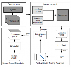
Figure 3: The proposed HPTA approach.
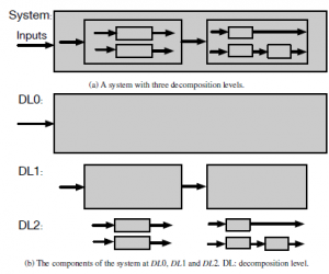
Figure 4: A system and the decomposition of the system at three decomposition levels.
4.1 Decomposition level
Figure 4a shows a system with components at three decomposition levels. The decomposition of the system is demonstrated in Figure 4b. Every grey rectangle represents one component, and the solid black arrows represent the data flow of the components. By our definition, DL0 is the lowest degree of decomposition because the complete system is measured at this level. The complete system is considered as one abstract component from which no details of the subsystems can be retrieved. At DL1, the mask of the system at DL0 is opened. Measurement can be conducted on the subsystems that are revealed at this level. As the decomposition level increases, the system is decomposed in further detail, more components are revealed. The decomposition level can increase until the last subsystem is opened. The granularity of the timing analysis increases with the decomposition level.
4.2 Challenges
4.2.1 Independent and identical data requirement
Although EVT requires the samples to be identically distributed, the adoption of GEV opened up the applicability of MBPTA to more cases because it can tolerate up to a certain degree of dependence in the measured execution times[10]. The disadvantage is that such dependence can corrupt the reliability of the derived pWCET [19]. In some domains, techniques such as re-sampling and de-clustering can be applied to create independence between measurements [20]. Nevertheless, forcing independence into dependent execution time measurements can result in overly optimistic pWCET that is not safe anymore [2].
For instance, the calculation in the example given in Section 3.1 is only valid when task A and B are independent, otherwise the result might be overly optimistic. Suppose dependence exists between the two events such that the execution time of task B is always 2 when the execution time of task A is 10. The probabilistic execution time when A and B are both executed would be:
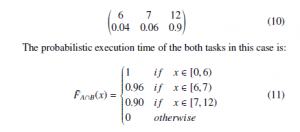
Given a deadline of 11, the probability of missing the deadline is 0.54 when A and B are independent (8), and 0.90 when A and B are dependent (11). In this case, overlooking the dependence between the tasks resulted in overly optimistic probabilities of a deadline miss.
4.2.2 Upper bound calculation
In deterministic hybrid timing analysis, the results are presented in absolute values. Therefore, the WCET of the complete system can be calculated simply by adding up the WCETs of every individual component. In statistics, convolution may be usually used to calculate the joint probability of two random variables. Unfortunately, this is not applicable in this context. The reason is that the probability distribution of the sum of two or more random variables is equal to the convolution of their distributions only when the variables are independent.
Since hybrid timing analysis is conducted on the components that construct the complete system, the execution time of one component often impacts the execution time of another component. This dependence makes the calculation of the overall pWCET much more complicated.
4.3 Solutions
Based on the information provided in the previous text, one can conclude that in order to overcome the challenges, we need to find a solution to the dependence in the measured execution times and the dependence between individual components.
4.3.1 Dependence in the observed execution times
In MBPTA and HPTA, dependence exists in the data samples if two or more of the observed execution times interfere with each other. Generally speaking, such dependence can come from:
- Software dependence: The dependence between inputs and the paths taken by the program. For example, if input/path A is always followed by input/path B, A and B are dependent.
- Hardware dependence: The hardware state left by the previous execution, which becomes the initial hardware state of the current execution.
To reduce the software dependence, we choose the per-path approach to collect the execution times for EVT. The other approach is know as the per-program approach [7]:
- Per-program: After the measurement, the EVT uses all the measured execution times as one sample group. EVT is applied to the sample group to estimate the pWCET for the complete program.
- Per-path: After the measurement, all the measured execution times are divided into sample groups. One group includes all the execution times measured from one program path. EVT is applied to each sample group to estimate the pWCET of the program path the sample group represents. The pWCET of the complete program is then calculated by taking the upper bound of the pWCETs of all the paths.
For instance, a system has two paths with the execution times at 10/15 (10 or 15 time units) and 60/65. The probabilities of the paths taken by one randomly chosen single execution are 0.3 and 0.7 respectively. Suppose the different execution times observed in the same path are due to a hardware component, which may generate 0 extra time units with a probability of 0.4 or 5 extra time units with a probability of 0.6. The probability execution time profile (ETP) of the system is:
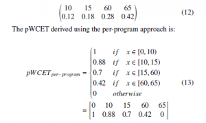

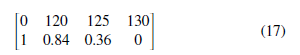
As can be seen, compared with the per-path approach, the perprogram approach was able to produce a tighter result. The pWCET derived using the per-program approach is valid to upper bound randomly chosen single executions of the target program. However, it is not applicable to be used in convolution when calculating the overall pWCET of multiple executions of the target program. The reason is that the probability distribution of the sum of two or more random variables is equal to the convolution of their distributions only when the variables are independent. For example, if path 60/65 is forced to be taken when path 10/15 is observed in the previous execution, the pWCET of two consecutive executions of the program is:

Under the dependence introduced by the execution condition, the probability that the two consecutive executions exceed 125 time units is 0.252. However, the pWCET using the convolution on the probability derived from pWCETper−program gives a probability of 0.1764, which is too optimistic.
In the per-path approach, the measured execution times are grouped according to the program paths. Therefore, the influence of the input data is eliminated within every group. The variations in the execution time within the same group are purely due to the hardware. By taking the upper bound of the pWCETs of all the paths, the pWCET generated by the per-path approach can be used safely in convolution for estimating any overall pWCET in which the execution of this task is executed consecutively. In the above example, the pWCET calculated by applying convolution to the probability derived from pWCETper−path is:
Therefore, using the per-path approach, the proposed HPTA method can upper bound the pWCET under the dependence introduced by the execution condition.
To reduce the hardware dependence, we try to push the hardware to the worst-case state at the beginning of every execution so that every execution can start with nearly the same initial state. For example, the pipeline is flushed, and “trash code” is executed to fill the caches with irrelevant data and instructions before every execution.
4.3.2 Dependence between components
In order to calculate the pWCET of the overall system using convolution, the independence between the pWCETs of the software components must be guaranteed. Such kind of dependence can be found in:
- Software dependence: The output of the precedent components, which is the input of the current component.
- Hardware dependence: The hardware state left by the previous component, which becomes the initial hardware state of the current component.
The software dependence can be removed together with the dependence in the observed execution times by the per-path approach. This is because the path-approach automatically selects the input(s) leading to the longest execution paths that upper bound all the other inputs. The hardware dependence no longer exists because the components execute in isolation from the rest of the program in the proposed method. Hence there are no precedent components.
5. Case study and experiment setup
5.1 Case Study
For the case study, we adopted a Simulink power window model.

Figure 5 is the power window model [21, 22] at DL0, DL1 and
DL2. A power window is an automatic window in a car that can be raised and lowered by pressing a button or a switch instead of a hand-turned crank handle. The complete application of a power window normally consists of four windows that can be operated individually. The three passenger-side windows can be operated by the driver with higher priority. In this paper, we only use the front passenger-side window and the driver-side window.
Figure 5: Power window passenger (left) and power window driver (right) at decomposition level 0, 1 and 2. DL: decomposition level; pw PSG: powerwindow passenger, De PSG: debounce passenger, CtrlEx: control exclusion, PW: powerwindow main component, De DRV: debounce driver, De: debounce, pw ctrl: powerwindow control, EP: end of range and pinch detection, D: delay.
The C code of the power window was generated using Embedded Coder R [23] targeting an ARM Cortex microprocessor with a discrete fixed-step solver at a fixed-step size of 5 ms. The BM approach with a block size of 20 was used in the extreme value selection process to collect the extremities for the EVT. The exceeding probability of 1E-10 was used for the pWCET.
The Kolmogorov-Smirnov (KS) test was used to verify the identical distribution requirement, and the runs-test was used to verify
Table 1: The p-values for the independent and identical distribution tests. NoN: number of nop instructions; pw DRV: powerwindow driver; pw PSG: powerwindow passenger; R: runs test; KS: Kolmogorov-Smirnov test.
| NoN |
pw DRV R KS |
pw P R |
SG KS |
NoN |
pw D R |
RV KS |
pw PSG R KS |
||
| 0 | 0.7495 | 0.9999 | 1 | 0.4973 | 8 | 1 | 0.7710 | 0.8486 | 0.1349 |
| 1 | 0.4019 | 0.2753 | 1 | 0.4973 | 9 | 0.3894 | 0.9999 | 0.6822 | 0.2753 |
| 2 | 0.9764 | 0.9999 | 0.4736 | 0.1349 | 10 | 0.2703 | 0.9655 | 0.3894 | 0.7710 |
| 3 | 0.3441 | 0.9655 | 0.8769 | 0.4973 | 11 | 0.9080 | 0.9655 | 0.3337 | 0.2753 |
| 4 | 0.7939 | 0.9655 | 1 | 0.1349 | 12 | 0.1065 | 0.7710 | 0.8052 | 0.7710 |
| 5 | 0.8046 | 0.7710 | 0.2003 | 0.2753 | 13 | 1 | 0.9999 | 0.0882 | 0.7710 |
| 6 | 0.5634 | 0.9655 | 0.1789 | 0.4973 | 14 | 0.5643 | 0.9999 | 0.3634 | 0.9999 |
| 7 | 0.6744 | 0.9655 | 0.2176 | 0.2753 | 15 | 1 | 0.2753 | 0.9687 | 0.4973 |
Table 2: The measured deterministic WCETs and the estimated probabilistic WCETs The exceeding probability of 1E-10 was used for the pWCET. of the complete powerwindow driver benchmark and the complete powerwindow passenger benchmark with 16 different alignments. NoN: number of nop instructions; pw DRV: powerwindow driver; pw PSG: powerwindow passenger; cc: clock cycles; dWCET: measured deterministic WCET; pWCET: estimated probabilistic WCET.
| NoN |
pw DRV (cc) dWCET pWCET |
pw PSG (cc) dWCET pWCET |
NoN |
pw DRV (cc) dWCET pWCET |
pw PSG (cc) dWCET pWCET |
||||
| 0 | 2516 | 2538 | 1638 | 1666 | 8 | 2660 | 2797 | 1678 | 1953 |
| 1 | 2656 | 2712 | 1660 | 1688 | 9 | 2650 | 2698 | 1674 | 1681 |
| 2 | 2514 | 2515 | 1664 | 1717 | 10 | 2586 | 2608 | 1650 | 1681 |
| 3 | 2764 | 2849 | 1672 | 1725 | 11 | 2700 | 2762 | 1648 | 1683 |
| 4 | 2712 | 2768 | 1640 | 1699 | 12 | 2748 | 2813 | 1646 | 1679 |
| 5 | 2708 | 2762 | 1642 | 1700 | 13 | 2646 | 2746 | 1646 | 1684 |
| 6 | 2726 | 2794 | 1666 | 1764 | 14 | 2620 | 2735 | 1670 | 1701 |
| 7 | 2714 | 2797 | 1670 | 1689 | 15 | 2568 | 2569 | 1632 | 1658 |
the requirement for independence. p > 0.05 indicates the data follows the desired distribution.
The case study is designed to test the following assumptions:
- Can the proposed HPTA method reduce the dependence in the measured execution times and facilitate the collection of i.i.d. execution times?
- Can the proposed HPTA method reduce pessimism at a higher decomposition level?
5.2 Experiment Setup
The experiment setup is shown in Figure 6. The processor is an
ARM Cortex-M7 processor that contains a four-way set-associative data cache and a two-way set-associative instruction cache. Both caches use the random replacement policy. The Xilinx Nexus 3
FPGA is used to measure the execution time of the code on the ARM-processor. It is driven by the CLK signal sent from the processor to synchronise the clocks. The measurement process starts by sending the Start signal from the FPGA to the processor. Two GPIO pins of the processor are used to set the Tic and Toc flags. Before the code starts to execute, the Tic pin is toggled to start counting the number of clock cycles that have passed. After the code is executed, the Toc pin is set to stop the timer. Eventually, the value in the timer (Execution Time) is collected through a serial port.

Figure 6: Experiment setup.
6. Results and discussion
6.1 Reducing dependence in the measured execution times
Table 1 shows the results of KS and runs test. As can be seen, all the p-values are significantly higher than 0.05, which means that the i.i.d. requirement is fulfilled and the collected data can be applied in EVT to estimate the pWCET. The NoN indicates the number of the nop instructions added to emulate different memory alignments [3]. These p-values confirm our assumption that the proposed HPTA can reduce the dependence in the executions to facilitate the collection of i.i.d. data required by the EVT.
6.2 Reducing pessimism in high decomposition levels
Across all the alignments, the estimated pWCET is more pessimistic at the selected exceeding probability compared with the deterministic WCET. However, in some cases, such as NoN = 15 in pw DRV, the difference between the two WCETs is relatively small. The reason could be that the execution time contributed by independent random elements in the hardware is reduced by imposing a worst-case execution scenario on the longest path. Since random events in the hardware rarely happen, the measured execution times can be very close to the estimated pWCET.
Table 3 shows the estimated pWCETs of the benchmarks calculated using sum and convolution at three decomposition levels. The highest pWCET of the 16 different alignments were used as the pWCET of every block. As can be seen, the WCETs increase with the decomposition levels. The highest WCET was reached by pWCETSum at DL2 with 6025 clock cycles for the driver and 3778 clock cycles for the passenger. The difference between the deterministic WCET and pWCETs also became more prominent with the decomposition and 1678 reached by NoN = 8 in the passenger-side window. The estimated pWCET in the driver-side window was 2849 reached by NoN = 3 and 1953 reached by NoN = 8.
Table 3: The estimated pWCET calculated using sum and convolution at different decomposition levels. DL: decomposition level; pw DRV: powerwindow driver; pw PSG: powerwindow passenger; cc: clock cycles; dWCET: measured deterministic WCET; pWCETSum: estimated probabilistic WCET calculated by adding the pWCETs of the components up; pWCETConv: estimated probabilistic WCET derived from the convolution of the pWCETs of the components.
The pWCET calculated using convolution (pWCETConv) is in general lower compared with the pWCETSum. Nevertheless, pWCETConv still leaves a reasonable margin with the determinis-
tic WCET. This observation confirms our assumption that simply adding up pWCETs in HPTA will lead to overly pessimistic results. Using convolution can help to reduce such pessimism and produce a reasonably sound result.
7. Conclusion
In this article, we proposed a HPTA method that is able to (i) collect the i.i.d. data required by EVT by reducing the dependence between the measured execution times and (ii) reduce the dependence between blocks to make it possible to use convolution to calculate the pWCET of the overall system. We are aware that forcing independence into dependent execution time measurements can make the data no longer representative of the dependent system behaviour. Therefore, several approaches, such as using the per-path approach to upper bound the pWCETs of all the paths, were taken to ensure the derived pWCET is not overly optimistic. However, this might have introduced too much pessimism into the estimated pWCET.
Another novelty of the proposed HPTA method is that it can be applied at different granularities by adjusting the decomposition level. Performing the analysis at a higher decomposition level can help to reduce pessimism. On the other hand, with the increased decomposition level, the cost to derive the pWCET also increases.
Compared with the deterministic HTA approach proposed in [3], this HPTA approach is more pessimistic with the exceedance probability of 1E-10. On the other hand, instead of giving a delevel, which means a higher decomposition level is associated with larger pessimism.
terministic value, this approach gives an exceedance probability to each possible execution time. We hope the results of this HPTA approach can be used as a reference to avoid unnecessary waste on the hardware cost in the hand of experienced engineers when designing a non safety-critical system that can tolerate a certain degree of deadline misses.
- L. Cucu-Grosjean, L. Santinelli, M. Houston, C. Lo, T. Vardanega, L. Kosmidis, J. Abella, E. Mezzetti, E. Quin˜ones, F. J. Cazorla, “Measurement-based probabilistic timing analysis for multi-path programs,” Proceedings – Euromicro Conference on Real-Time Systems, 91–101, 2012, doi:10.1109/ECRTS.2012.31.
- F. Guet, L. Santinelli, J. Morio, “On the representativity of execution time measurements: Studying dependence and multi-mode tasks,” in OpenAccess Series in Informatics, volume 57, 31–313, Schloss Dagstuhl-Leibniz-Zentrum fuer Informatik, 2017, doi:10.4230/OASIcs.WCET.2017.3.
- H. Li, K. Vanherpen, P. Hellinckx, S. Mercelis, P. De Meulenaere, “Component-based Timing Analysis for Embedded Software Components in Cyber-Physical Systems,” in 2020 9th Mediterranean Conference on Embedded Computing, MECO 2020, 1–8, IEEE, 2020, doi:10.1109/MECO49872.2020.9134177.
- H. Li, P. De Meulenaere, K. Vanherpen, S. Mercelis, P. Hellinckx, “A hybrid timing analysis method based on the isolation of software code block,” Internet of Things, 11, 100230, 2020, doi:10.1016/j.iot.2020.100230.
- R. Wilhelm, J. Engblom, A. Ermedahl, N. Holsti, S. Thesing, D. Whal- ley, G. Bernat, C. Ferdinand, R. Heckmann, T. Mitra, F. Mueller, I. Puaut, P. Puschner, J. Staschulat, P. Stenstro¨ m, “The worst-case execution-time problem-overview of methods and survey of tools,” Transactions on Embedded Computing Systems, 7(3), 36:1–36:53, 2008, doi:10.1145/1347375.1347389.
- L. Santinelli, F. Guet, J. Morio, “Revising measurement-based probabilistic timing analysis,” in Proceedings of the IEEE Real-Time and Embedded Technology and Applications Symposium, RTAS, 199–208, IEEE, 2017, doi: 10.1109/RTAS.2017.16.
- R. Davis, L. Cucu-Grosjean, “A Survey of Probabilistic Schedulability Anal- ysis Techniques for Real-Time Systems,” LITES: Leibniz Transactions on Embedded Systems, 6(1), 1–53, 2019.
- J. Hansen, S. Hissam, G. A. Moreno, “Statistical-based WCET estimation and validation,” OpenAccess Series in Informatics, 10(January), 123–133, 2009, doi:10.4230/OASIcs.WCET.2009.2291.
- F. J. Cazorla, T. Vardanega, E. Quin˜ones, J. Abella, “Upper-bounding program execution time with extreme value theory,” in OpenAccess Series in Informat- ics, volume 30, 64–76, Schloss Dagstuhl-Leibniz-Zentrum fuer Informatik, 2013, doi:10.4230/OASIcs.WCET.2013.64.
- L. Santinelli, J. Morio, G. Dufour, D. Jacquemart, “On the sustainability of the extreme value theory for WCET estimation,” OpenAccess Series in Informatics, 39(July), 21–30, 2014, doi:10.4230/OASIcs.WCET.2014.21.
- F. J. Cazorla, J. Abella, J. Andersson, T. Vardanega, F. Vatrinet, I. Bate, Broster, M. Azkarate-Askasua, F. Wartel, L. Cucu, F. Cros, G. Farrall, A. Gogonel, A. Gianarro, B. Triquet, C. Hernandez, C. Lo, C. Maxim, D. Morales, E. Quinones, E. Mezzetti, L. Kosmidis, I. Aguirre, M. Fernandez, M. Slijepcevic, P. Conmy, W. Talaboulma, “PROXIMA: Improving Measurement-Based Timing Analysis through Randomisation and Probabilistic Analysis,” Proceedings – 19th Euromicro Conference on Digital System Design, DSD 2016, 276–285, 2016, doi:10.1109/DSD.2016.22.
- S. Trujillo, R. Obermaisser, K. Gru¨ ttner, F. J. Cazorla, J. Perez, “European Project Cluster on Mixed-Criticality Systems,” in Design, Automation and Test in Europe (DATE) Workshop 3PMCES, 2014.
- M. Schoeberl, S. Abbaspour, B. Akesson, N. Audsley, R. Capasso, J. Gar- side, K. Goossens, S. Goossens, S. Hansen, R. Heckmann, S. Hepp, B. Huber, Jordan, E. Kasapaki, J. Knoop, Y. Li, D. Prokesch, W. Puffitsch, P. Puschner, A. Rocha, C. Silva, J. Sparsø, A. Tocchi, “T-CREST: Time-predictable multi- core architecture for embedded systems,” Journal of Systems Architecture, 61(9), 449–471, 2015, doi:10.1016/j.sysarc.2015.04.002.
- L. Kosmidis, J. Abella, E. Quinones, F. J. Cazorla, “A cache design for proba- bilistically analysable real-time systems,” Proceedings -Design, Automation and Test in Europe, DATE, 513–518, 2013, doi:10.7873/date.2013.116.
- J. Jalle, L. Kosmidis, J. Abella, E. Quinon˜es, F. J. Cazorla, “Bus designs for time-probabilistic multicore processors,” Proceedings -Design, Automation and Test in Europe, DATE, 1–6, 2014, doi:10.7873/DATE2014.063.
- I. Fedotova, B. Krause, E. Siemens, “Applicability of Extreme Value Theory to the Execution Time Prediction of Programs on SoCs,” in Proceedings of International Conference on Applied Innovation in IT, volume 5, 71–80, Anhalt University of Applied Sciences, 2017.
- Y. Lu, T. Nolte, J. Kraft, C. Norstro¨m, “Statistical-based response-time analysis of systems with execution dependencies between tasks,” in Proceedings of the IEEE International Conference on Engineering of Complex Computer Systems, ICECCS, 169–179, IEEE, 2010, doi:10.1109/ICECCS.2010.26.
- H. Hersbach, “Decomposition of the continuous ranked probability score for ensemble prediction systems,” Weather and Forecasting, 15(5), 559–570, 2000, doi:10.1175/1520-0434(2000)015(0559:DOTCRP.2.0.CO;2.
- F. Guet, L. Santinelli, J. Morio, “On the Reliability of the Probabilistic Worst- Case Execution Time Estimates,” European Congress on Embedded Real Time Software and Systems 2016 (ERTS’16), 10, 2016.
- J. Segers, “Automatic declustering of extreme values via an estimator for the extremal index Automatic declustering of extreme values via an estimator for the extremal index,” (April 2002), 2014.
- H. Li, P. De Meulenaere, P. Hellinckx, “Powerwindow: A multi-component TACLeBench benchmark for timing analysis,” in Lecture Notes on Data En- gineering and Communications Technologies, volume 1, 779–788, Springer, 2017, doi:10.1007/978-3-319-49109-7 75.
- H. Li, P. De Meulenaere, S. Mercelis, P. Hellinckx, “Impact of software architecture on execution time: A power window TACLeBench case study,” International Journal of Grid and Utility Computing, 10(2), 132–140, 2019, doi:10.1504/IJGUC.2019.098216.
- “Embedded Coder,” 2020.