1. Introduction

Advances in Science, Technology and Engineering Systems Journal installed to satisfy the demands of modern lifestyles. It has led to instability of the power system, creating high noise levels in the system grids and decaying the electrical distribution system. Even This paper is an extension of work originally presented in the confer- worse, climate change has an impact on the environment that the ence Proceedings of the 2019 IEEE/SICE International Symposium system operates in. In some cases, particularly for hot countries, the on System Integration (SII) [1]. Power Quality (PQ) monitoring electrical distribution system requires air conditioning to protect the ^{has been the focus of research and development for many years.} electrical equipment in the substation. In normal circumstances, if Recently, [2], [3] addressing the PQ issues in various industry and the air conditioning fails, it may surpass the permitted set point and proposing different methods in tackling this issues.The main focus may not protect the equipment. When the global temperature rises, ^{is to protect the equipment and minimize the losses while increasing} the potential rate of failure also increases. Research has shown that ^{the levels of operational safety. However, systems are becoming} the long-term average global temperature is increasing, which has a ^{more complex as they are being further developed for improvement.} significant negative impact on the performance of the machines [4]. Huge numbers of control drive and other non-linear loads have been

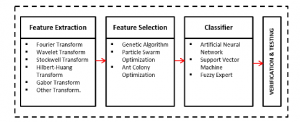
Figure 1: Various techniques of Power Quality Classification

The arrangement of the three principal stages in PQ Classification: (1) Feature extraction – a key transformation of the fundamental signals into time-frequency based information. A broad selection of Fourier Transform, Wavelet Transform, Stockwell Transform, Hilbert-Huang Transform, Gabor Transform and others. (2) Feature Selection – a key method in selecting the most suitable features from the feature extraction stage while discarding the redundant features. Few main optimizers include

Genetic Algorithm, Particle Swarm Optimization and Ant Colony Optimization. (3) Classifier – a selection of artificial intelligence tools in classifying PQ disturbances such as artificial neural network, support vector machines, and fuzzy expert.

Earlier, conventional methods use manual configurations and visual inspection to monitor the quality of the power supply in the system. This method was too difficult to interpret and timeconsuming. Later, an automated classification system, which uses the signal processing technique was developed and currently advancing with various Machine Learning and Deep Learning approach. Various combinations of features extraction and classifiers have proven to locate PQ disturbances accurately while using synthetic data. However, this is not the case with real industry data. Real industry data are complex and much more complicated when there are external or environmental factors that could potentially influence the state of the system. This creates a gap in existing techniques, which motivates authors to investigate the relevance of the environmental parameter to the issue of PQ disturbances. In addition, with the current emergence of big industrial data, system engineer must ensure that the system is robust and capable of performing ML/DL techniques in real-time applications. Disturbance data exists in the order of microseconds, which greatly enhances the record data [5].In consequence, it will burden learning classifiers to run unimportant parameters that result in high computation. The authors, therefore, suggest a method that could minimize the dimensional by selecting the most relevant data to be trained automatically, while incorporating a new unknown parameter that was previously considered irrelevant in the system state.

The aim of this paper is to introduce event-based analysis as a technique for detecting harmonic failure in real time. The technique is capable of grouping together high correlation system parameters, forming an input-output relationship that is not limited to internal parameters only. As such, the homogenized correlation system will indicate the possible root cause of harmonic failures, while eliminating non-important parameters in real-time [6]. This paper presents a real-time simulation of CSU machines, which shows the changes in the output parameters of the input activity. The data will be used to measure the suitability and applicability of event modelling techniques in the power system environment. It is then extended to the actual plant data, exploring the integration of this dynamic platform with the Key Performance Indicator (KPI) in order to recognize the system operating pattern. This data analytics technique expects to predict the homogenized system parameter that could present the current state of the system in real time.

1.1     Power Quality Disturbance

A number of PQ disturbance types are implicated: voltage sag, voltage swell, transients, harmonics, fluctuations, flickering, voltage imbalance, interruption, DC offset and notches. A high level of engineering expertise [7] is needed to effectively diagnose these PQ disturbances. Preventing PQ disturbances is critical to minimize power interruptions between the power utility and the end user. With modern technology, a substantial amount of research has been devoted to alleviating these problems using signal processing technique. This technique has three principal stages which incorporate feature extraction, feature selection and classification.

Feature extraction is a key transformation of the fundamental signals into time-frequency based information. It can be extracted directly from the original measurement either from a transformed domain or from the signal model parameters [8]. Several approaches include short-time Fourier transform [9], wavelet transform [10], wavelet packet transform [11], Hilbert Huang transform [12], Stockwell transform [13], Gabor-Wigner transform [14], and other hybrid transform-based [15].

Feature selection is a key method in selecting the most suitable features from the feature extraction stage while discarding the redundant features. Based on the extraction data, optimization techniques such as Ant Colony Optimisation [16], Genetic Algorithm [17], and Particle Swarm Optimisation [18] are the common algorithm used in locating PQ disturbances.

Classification is the process of predicting the class of data points. It uses an algorithm to implement classification by approximating the mapping function from the input variable to the output variable. One of the most popular and influential types of machine learning algorithms is the Artificial Neural Network. Other machine learning includes Support Vector Machine [19] and fuzzy expert system [20]. Figure 1 illustrates the three main phases of the PQ classification. [21]–[22] provide a detailed review of these techniques.

1.2    Power Quality Standards

Harmonic assessments of utility systems require procedures in place to ensure that the efficiency of the voltage supplied to all consumers is adequate [23]. However, most of the harmonic issues arise at the end of the consumer. Their devices contain non-linear loads resulting in resonance conditions [23]. These non-linear loads are the current harmonic sources. The system voltage appears stiff to individual loads, and the loads draw distorted current waveforms. It is therefore important to maintain the PQ International standard, to provide the guidelines and limits for the acceptable levels of compatibility, between consumer equipment and the system utilities.

The International Standard IEEE 519-1992 sets the limit for both harmonic voltages and currents at the Point of Common Coupling (PCC) between the end-user and the utility supplier. It limits Voltage Total Harmonic Distortion (THD), defined as the ratio of the RMS value of the harmonic voltage to the RMS value of the fundamental (50Hz) voltage, to a maximum of 5%. Individual voltage harmonic magnitudes are limited to 3% of the fundamental voltage value [24]. The International Standard IEC 61000-3-4 sets the limits for the emission of harmonic currents in low-voltage power supply systems for the requirement with rated current greater than 16A [25].

1.3    Environmental Parameters

Compliance with the International PQ Standards is the policy for both utilities and customers. In order to maintain a good PQ system, an enormous amount of research and PQ analysis has been undertaken to ensure it complies with the standards. However, in some cases, the machine still fails, although it complies with the standard. It is important to note that most of these research focuses on the fundamental of the electrical system and leave behind the external parameters that may have a substantial effect on the problem. In [26], the authors suggest that there could be further environmental and operational factors that could also affect the performance of power systems.

1.4    Problem Statement

In this article, we intend to investigate what possible factors that could link a well-maintained machines with a proper operation to a frequent harmonic failure incidents. While PQ parameters are eliminated by its healthy measurement, an alternative technique to solve this harmonic failure mystery is required to evaluate if there is an existence of a different parameter that could lead to this failure. Therefore, the authors are proposing the Event Modeller techniques which could link the internal and external parameters together, to create a cause-effect relationship, while updating the system status in near real-time before the machine fails. The implementation of the event modeller technique recently has shown positive practical findings in various area and application such as high-speed causal prediction modelling [27, 28], real-time Remaining Useful Life (RUL) estimation [29], and as a middleware to highly coupled input variable in zero-defect manufacturing [30], and predicting N₂O Emission [31].

1.5    Contribution & Advantages

The first contribution of this paper is to proposed a robust system engineering tools that be able to formulate a piece of new knowledge information in the diagnosis of PQ disturbances in real-time. This tool is found robust, workable with the dynamic and autonomous environment while being able to withstand real industry data which is non-linear and highly influenced with various factors. The second contribution of this paper is that the proposed technique could visualize the group of highly correlated variables in the form of occurrence matrices in real-time, proposing a mathematics equation that represents the current state of the system. This is optimum to system operators who can make a quick decision before the system fails.

1.6    Challenges

However, implementing this technique in solving PQ problems has its challenges. The harmonic readings (THD) is taken from the Multi-Function meter, which is installed at the electrical switchgear.

The reading will not be as accurate as of the conventional method, but the measurement is sufficient to prove that the PQ parameters can be eliminated. Another challenge is to determine the threshold setting. In general, a scenario of events in the actual system varies according to the system characteristic and its system deterministic. An event could happen instantaneously, or it may have some delay before it reached to the target output. For example, the scenario of a room temperature does not change immediately when the heater or air conditioner was switched on. In comparison, a dark room will be immediately bright when the switch was turned on. Both of the scenarios have made changes to the system state at a different pace. In order to detect this, a data benchmarking is required which were decided based on historical data and system expert point of view.

2. Event Modeller Technique

The event modeller technique is designed to investigate the association between the observable events (Output Data) with the causal events (Input Data) through a data mapping concept [30]. It clusters the system parameters with the highest correlation in the form of matrices and places them into mutually exclusive blocks. This creates an input-output relationship, which considers both internal and external factors. One significant difference between the proposed event modeller and other traditional data modelling techniques is how the input data assumes its output data. The traditional method assumes the input-output relationship as a true representation of a known data series, while the event modeller technique makes no assumption about it (unbiased) [32]. This fundamentally makes the approach non-unbiased vis-a-vis input-output relationship. The` proposed Event Modeller Data Analytic (EMDA) is designed to find any interceptions between the known influential parameters (reported in previous literature) and new operational and environmental data by expanding the spectrum and reassessing the relationship between influential parameters on harmonic behaviour. It is a proven, computationally effective method of analyzing harmonic behaviour without bias. Borrowing from the Event Tracker [33] and Event Clustering [34] method, the proposed EMDA extends the previous authors’ correlation map by adding the information from the machine performance metrics. Information such as machine availability, utilization and performance are combined with other technical data, to group the highly correlated individual data together, revealing the machine’s status in real-time. Figure 2 illustrates the event modeller techniques, including Event Tracker, Event Clustering and a Look-up table. Details of each stage will be briefly discussed in the following subsection.

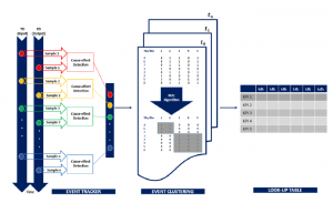
Figure 2: Event Modeller Techniques

The arrangement of the three principal stages in Event Modeller: (1) Event Tracker – A collection of input-output cause-effect detection of a system state with highly sensitivity index in real-time. (2) Event Clustering – A rank order grouping technique based on the interpretation of the changes of input-output data in the previous stage.

(3) Look-up Table – A population table that links the Key Performance Indicator with the Sensitivity Indexes.

2.1        EventTracker Algorithm

EventTracker algorithm was introduced [35] to construct a discrete event framework for online sensitivity analysis (SA). This algorithm was designed to be applied to highly volatile environments with real-time scalar data acquisition capabilities (e.g. Internet of Things (IoT). It uses a cause-effect detection algorithm to dynamically track events’ triggers and their interrelationship with one another in a given system. It generates a sensitivity index that measures the relationship between the triggered data and the event data pairs. High sensitivity index score will be indicated while the lesser impact relationship will be eliminated. This will reduce the computational effort while achieving dimensional reduction. The Event Tracker is a computationally efficient technique that focuses on the state changes of the involved system components. It merely takes a snapshot of the system states, which helps engineers observe system performance [6]. Further details on the description and four EventTracker functional parameters (Search Slot, Analysis Span, Event Threshold and Trigger Threshold) can found in [35].

2.2        Event Clustering Algorithm

Event Clustering Algorithm (EventiC) [34] is designed to improve the real-time sensitivity analysis, by automatically re-arranging the input-output relationship in rank order of its importance and relevance. The algorithm applied the Rank Order Clustering (ROC) technique, which was initially introduced in [36]. This technique interprets the changes in input-output data’s value at the given level, detecting the coincidence and finally groups it as a related event. The process of calculating the number of coincidence occurs at a specified scan rate time interval, to ensure a relationship weight is established for modelling and control purposes [32]. Despite filtering the unimportant relationship between the input-output relationship, event clustering can identify new influencing parameters that were previously thought irrelevant, making it unique and interesting to improve the data quality. One key advantage of EventiC compared to EventTracker is that EventiC can assess multiple input/ output relationship in every single scan, whilst EventTracker considers multiple input single output relations. A detailed explanation of EventiC algorithm and the basic concept is discussed in [34]. Algorithm 1 shows the main procedure of Event Modeller.

2.3        Look-up Table

A look-up table is an array of data to map input values to output values. It is used to transform the input data into a more desirable output format. The look-up table allows replacing run-time computation or logic circuitry with a simpler array indexing operation [37]. Retrieving a value from a look-up table is faster rather than examining it from the whole database. With the advantage of the logical separation of data, it makes it relevant to prepare the data for machine learning purposes. This EMDA technique’s novelty can be found in this look-up table, thus a rapid response to changes in the system’s stability (i.e. the KPIs).

Algorithm 1: Event Modeller

Set Event Modeller Limit (EML);

Set Threshold Setting (Th);

Populate ULTh and LLTh; Populate All Input Data (TD1, TD2…TDn); if Triggered Data = Dynamic TD then

Compute TDx = TDn – TDn-1; Compare TDx with ULTh and LLTh; if (LLTh<TDx<ULTh) then

TDx = 0;

TDx = 1;

Triggered Data = Static TD;

TDx = TD1,TD2…TDn.;

Populate All Output Data (ED1,ED2…EDn);

Compute EDx = EDn – EDn-1; Compare EDx with ULTh and LLTh; if LLTh<EDx<ULTh then

Set EDx = 0; else

Set EDx = 1; end

Populate the models input-output event coincidence matrix with binary weighting values of exclusive NOR function;

Average each input-output event coincidence; Sort rows of the resultant binary matrix into decreasing order of their decimal weights;

until for every column; until position of each element in each row and column does not change;

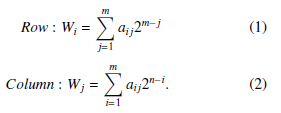
Calculate the weight for each row i and column j (in a m by n matrix) using Equation 1 and Equation 2.

the KPIs for brewery industry. In [39] the author used data-driven scheme of KPIs prediction and diagnosis for hot strip mill industry. In [40], the author proposes an analytics solution for calculating statistical KPIs in the Human Machine Interface (HMI) layer. There is a need to translate a suitable KPI that suit the type of operation. Basic KPIs are calculated directly from the output operation data, and they serve as the foundation for Overall performance KPIs [41].

Time-based KPIs are data related to time duration, defining activities associated with production and maintenance. The calculation of KPI has to consider all these factors to reflect accurate metrics. Hence it is important to understand the KPI interrelationship. A hierarchical structure for KPI categorization is proposed by [41]. The time-based KPIs studied in this paper are Availability, Instantaneous Utilization, Schedule Utilization and Performance.

To complement the Time-Based KPIs, it is useful to look at the energy consumption and emission contribution that could potentially harm the environment. In general, energy consumption can be calculated by multiplying the motor rating (kW) with the duration it operates. There are three states of motor known as run, idle and stop. During running state, the motor is capable of operating at its 100% loading while in idle state, the motor operates at 25% of its loading. Obviously, there is no loading when it stops. Having the total energy consumption, it is easier to calculate the carbon footprint; Carbon Dioxide Emissions (kgCO^[1], kgCO₂e), Methane (kgCH₄) and Nitrous Oxide (kgNO₂) using the formula in [42].

3. A Case Study

A Continuous Ship Unloader (CSU) is one of the leading bulk material handling machine. In a coal-fired power plant, this machine is used to transport coal from the vessel to the pulverized boiler through a series of belt conveyors. It has been reported that the CSU machine in one of the power plants in Malaysia has a frequent harmonic failure. The repetitive incidents lead to catastrophic failure, which harms the electrical devices. Besides having a vast replacement cost for the faulty parts, it is also affecting the plant availability, which concerned the management team. Even worse, it could pose a potential hazard, to the personnel working in the area if it is happening again in the future. A thorough Power Quality (PQ) assessment within the electrical distribution system has been assessed, but the results have not given any indication of internal disturbance or fault. Table 1 shows the assessment result for the CSU machine. To mitigate the problem, an effort to analyze both internal and environment parameter that has a significant impact on the system is highly desirable. The authors are keen to embrace the event modeller techniques, to evaluate the significant correlation between the output and input, which could cause harmonic failures in the system. A real-time simulation which incorporates the CSU machine parameters and the event modeller algorithm was developed using National Instruments LabVIEW.

3.1        Experiment 1: CSU Real-time Data Simulation

Table 1: Assessment Results for CSU Machine Parameters Units Min Max Avg Voltage Vab Vbc 385.9 V 216.8 V 424.0 V 423.8 V 411.2 V 382.4 V Vca 241.8 V 424.1 V 381.5 V Current Ia Ib 32 A 46 A 1718 A 1870 A 525.8 A 639.9 A Ic 30 A 1568 A 217.6 A Voltage Unbalance % Unbalance 0.10 % 41.60 % 2.60 % Current Unbalance % Unbalance 8.80 % 16.70 % 52.80 % Total Harmonic Distortion Voltage (THDV) THDvab THDvbc THDvac 0.40 % 0.30 % 0.50 % 1.60 % 1.50 % 1.90 % 1.00 % 1.00 % 1.10 % Total Harmonic Distortion Current (THDi) THDia THDib THDic 1.90 % 1.80 % 1.90 % 20.80 % 25.80 % 82.20 % 4.50 % 3.70 % 12.00 % Total Demand Distortion Current (TDDi) TDDia TDDib TDDic 0.10 % 0.10 % 0.10 % 2.60 % 1.80 % 2.20 % 1.30 % 1.20 % 0.80 % Frequency f 49.77 Hz 50.13 Hz 49.98 Hz

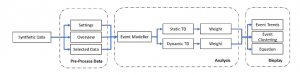
Figure 3: Experiment Strategy for Event Modeller Simulation

The arrangement of the three principal stages in the Experiment Strategy for Event Modeller Simulation: Pre-process Data, Analysis and Display.

The purpose of a real-time simulation is to measure the suitability and applicability of the event modeller technique in the power system environment. To ensure the system incorporates the industrial case study, the requirement specification has been set based on the following:

1. 8 Event Data (ED’s). This synthetic event data is simulated using Normal Distribution which represents the CSU Machine Output Data which includes Voltage, Humidity, Harmonics,

Slewing Movement, Luffing Movement, Travel Movement, Temperature and Wind Speed;

2. 8 Triggered Data (TD’s). This synthetic TD’s is simulated using Normal Distribution which represents the CSU Machine Input data which includes Busy Slew, Busy Luff, Busy Travel,

Busy Bucket Elevator, Slewing Motor Run Bit, Hydraulic Motor Run Bit, Travel Motor Run Bit and Bucket Motor Run Bit;

3. Threshold Setting. For the purpose of examining the Trigger Threshold, an arbitrary 5% threshold setting was set, that could later be adjusted;
4. Event Modeller Limit. This setting reduces the complexity

of an input-output relationship by its correlation confidence level. An arbitrary 80% was set, that could later be adjusted;

3.1.1       Experiment Strategy

Sixteen input/output system parameters of a CSU Machine were sampled from the Allen Bradley PLC-SCADA system using the FactoryTalk view. Once it is proven to be suitable, it will be extended to 120 parameters, which will be discussed further in Section 3.2. Data collection was conducted over a single day shift of a machine operation period, collecting approximately 43,200 lines of 12-hour data samples.

The sampling frequency follows [43] by applying the right bandwidth, time constant and settling time. Having this data in hand, synthetic data was constructed to have the same nature and properties as the real CSU machine. The overview of the experimental methodology is shown in Figure 3. Details of the dataset arrangement will be discussed in the following section.

Table 2: CSU Real-time Data Simulation Results (Weight) Based on Disturbance Description Voltage Humidity Harmonic Temperature Wind Speed Static Dynamic Static Dynamic Static Dynamic Static Dynamic Static Dynamic Overall Maximum 0.8387 0.9996 0.8364 0.9996 0.8370 0.9997 0.8360 1.0000 0.8340 1.0000 Overall Minimum 0.5000 0.6288 0.5000 0.6371 0.5000 0.6360 0.5000 0.6312 0.5000 0.6325 k-Disturbance (Pre) 0.8345 0.9890 0.8287 0.9790 0.8181 0.9791 0.8306 1.0000 0.8424 1.0000 k-Disturbance (Dur) 0.7615 0.8065 0.7781 0.8304 0.7637 0.8137 0.7977 0.8976 0.7848 0.8103 k-Disturbance (Post) 0.7813 0.8667 0.8011 0.8789 0.7897 0.8650 0.8087 0.9310 0.8035 0.8654

3.1.2       Dataset Arrangement

ED is defined as a series of data that represent the state of the system at a given time [35]. In this simulation, the ED consists of simulated voltage, humidity, harmonics, machine positioning (slewing, luffing and travelling), temperature and wind speed. The simulation data is based on the actual operation and environment data of the CSU machine events by considering the assessment result in Table 1 and the location of the power plant located in Malaysia. The plant is located near to the seaside, which is hot and humid throughout the year and may tend to have strong winds. On the other hand, the machine movements are simulated based on the 3-axis movement, which includes slew (x-axis), luffing (y-axis) and travel (z-axis).

In Discrete Event System, any input variable whose value transition register as an event is defined as a TD [35]. In this simulation, the TD consists of machine status (slewing, luffing, travel and bucket) and motor run feedback (slewing, hydraulic, travel and bucket). For comparison purposes, two types of TD are presented here known as Static TD and Dynamic TD. Static TD registered the original TD signal from the source while Dynamic TD multiply the changes of TD with a threshold setting defined by the system engineer. Both types of TDs were used in this experiment to investigate which source of data to be selected. This will ensure the event modeller algorithm provides an accurate sensitivity index or weight output.

Meanwhile, the threshold level could be adjusted based on the expert point of view. In this simulation, the threshold level is set at 5% (0.05); thus, the Upper Limit and Lower Limit will automatically set to 1.05 and 0.95 consecutively. The limits will be multiplied to the individual data computationally, to calculate the changes of the current data to the previous data and reflects the algorithm for weight score using X-NOR logic. The event modeller limit is the desired weight limits which also could be adjusted based on the expert point of view. In this simulation, the event modeller limit is set at (0.8). The weights who score above the Event Modeller Limit is shaded in the ROC Output table, indicates a significant correlation between the ED and the TD.

The sequence of TD’s and ED’s is updated every second and are re-arrangeable according to the weighted score. The weighted score can take a value of 0.5 and 1. The value is 1 when both or none of the input/output are triggered. Otherwise, it is 0.5. The weighted score is then averaged based on the number of iteration. Having the weight score in real-time, system engineers could easily notify the management team if there is any disturbance occurs in the system state by looking at the sequence and the weights. For trending purposes, a waveform chart is presented to improve the visibility of the data.

3.1.3       Disturbance Signal

The purpose of this simulation is to test the applicability of the Event Modeller algorithm in the handling of real-time data, thus observing the reaction of the system to the abnormal events. To ensure the system is sensitive to this abnormality, a k-Disturbance signal is introduced to the system. In this simulation, the data is simulated in 3 stages known as pre-disturbance, k-disturbance and post-disturbance. The pre-disturbance refers to the warm-up stage, which represents the machine normal steady state. The kdisturbance refers to the fluctuation of the k-event data, in such generating disturbance to the system. The post-disturbance refers to the reaction of the abnormal system back to normal steady state. A 5 minutes time interval is selected for each stage, which accumulates to 15 minutes of sampling time.

In this simulation, 5 ED’s signal, which represents the internal and environment parameter, has been chosen to be disturbed. This includes voltage, humidity, harmonic, temperature and wind speed. The signal data are simulated based on random fluctuation with 5% disturbance limit from normal operation data capability.

3.1.4       Simulation Results

Table 2 compares the results obtained from the simulation of the CSU machine against the k-disturbance signal. To present the findings, the performance is measured from the score of the sensitivity index from two main perspectives, which includes the overall maximum and minimum weight, and the average score for each stage. What stands out in the table is that the value of the weight has changed drastically between the pre-disturbance and during disturbance for all case. For e.g., when the k-disturbance is applied to the machine voltage using Static TD, the weight value drops from 0.83450 to 0.76154. However, when the k-disturbance is removed, the weight value rose to 0.78132. These indicate that the system parameters are sensitive to the disturbance signal introduced in the system.

It is interesting to note that all ten cases of this study have a common finding. The transition of average sensitivity index (weight) from Pre-Disturbance to k-Disturbance have the same reduction trend with an average of 8.2% reduction for Static TD and 15.94% reduction for Dynamic TD. Alternatively, when the k-Disturbance recovers, there is also a trend of increased weight with an average of

3.218% increment for Static TD and 6.023% increment for Dynamic TD. This finding confirms the interrelation between the triggered data and the k-disturbance event data, where different TD types have different performance. The Dynamic TD has a higher percentage of changes compared to Static TD.

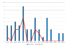
Figure 4: Tabulation of CSU Machine Failure vs REGEN Failure

The bar chart reveals that the highest number of REGEN faults was reported in October 2018, followedby August 2018, September 2018 and January 2019 consecutively.

On the other hand, it has been observed that the minimum weight for Static TD is fixed at 0.5000 while Dynamic TD has different minimum weight scores for each experiment. A possible explanation for this might be that the Dynamic TD captured the changes of input sensitivity rather than a direct Boolean signal from the input itself.

3.2       Experiment 2: CSU Real-time Machine Failure Analysis with KPIs

Harmonic filter failure can be influenced by various factors, such as faulty device, operator handling, and environmental factors in which the machine operates. It has also occasionally been affected by the combination of these factors. Based on the CSU machine expert point of view, the harmonic problem is associated with the occurrence of Regenerative Drive (REGEN) fault. In order to access the REGEN fault events, the abnormal dataset was selected. The frequency of the REGEN failure was compared with other types of fault, as presented in Figure 4. The bar chart reveals that the highest number of REGEN faults was reported in October 2018, followed by August 2018, September 2018 and January 2019. Although the highest number of REGEN failures was recorded in October 2018, no report indicated that the REGEN drives had been replaced. However, the January 2019 reports indicated that the maintenance team had replaced the REGEN during this month due to a fault. The January dataset was therefore chosen to further explain the relationship of the variables using the proposed technique.

3.2.1       Experiment Strategy

Building a solution capable of translating engineering data automatically into high-level management information is the principal motivation for this experiment. The KPIs shall be calculated based on the operation of the machine during the selected period. The method used in [1] is borrowed to run a fault dataset with a time interval of 5 minutes. The first 5 minutes are the events before the fault occurs, followed by the fault, and end with the last 5 minutes that accumulate up to 15 minutes of sampling time. The reason why this method was adopted is to prove that the event modeller could instantly solve a complex system without having to run the system for a longer period. It is easy to sample data in a simulation environment, as the user can decide when the fault may occur, but this is not the case with industrial data. The dataset was therefore analyzed to determine which data was almost equivalent to the setting. The experiment strategy is summarised in Figure 5. The results are presented in two phases. First, the event modeller was used as a tool to reduce the dimensionality of the data being observed. Second, the relationship between the observed data and the KPIs has been compared. The results will be explained as follows.

3.2.2       Dataset Arrangement

In this example, a homogenous dataset representing REGEN failure of the predictive model population was sampled for 16 minutes. The dataset of 30^th January 2019 was sampled between 12:47 pm and 13:03 pm. The dataset arrangement indicated that there were 96 TDs to be grouped against 24 EDs in the form of matrices to show which system parameters were highly correlated. It is noteworthy that the 96 X 24 matrices are too complex for a correlation analysis; therefore, the 96 TD was divided into 4 clusters. For each TD cluster, 24 X 24 matrices were analyzed using the event modelling technique.

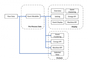
Figure 5: Experiment Strategy for KPIs Analysis

The arrangement of the three principal stages in the Experiment Strategy for KPI Analysis: Pre-process Data, Analysis and Display.

The sensitivity index of each input-output relationship has been measured and updated every second. The ROC pattern was observed in real-time and captured every minute. As a result, four-quadrant windows representing four key states were presented: Initial, PreFault, Fault and Post Fault for each TD cluster. This analysis intends to examine how TDs influence the pattern of the ROC. It is necessary to clarify what happens during this 16-minute time stamp before presenting the chart. Based on the report, the machine is running at its optimum level before it is fully phased out after 10 minutes. The reason why machine trips are unknown, which left the proposed method to be concluded further.

3.2.3       Dimensionality Reduction using Event Modeller

One advantage of using Event Modeller is to reduce the dimensionality of a complex system. As the main objective is to identify the root cause of the failure, this technique is capable of highlighting the ROC pattern based on its correlation analysis. One important finding was that the first four EDs were the same for all clusters. They comprised of E-House Humidity (ED24), Portal Conveyor Current (ED18), Wind Speed (ED 12) and Portal Speed Drive (ED14). This indicates that one of these EDs would have been the cause of failure. However, it has been noted that Cluster 2 and Cluster 3 consistently remain the same pattern with or without fault happened.

Therefore, we have eliminated Cluster 2 and Cluster 3 from the analysis. Moving to the ROC patterns for Cluster 1 and Cluster 4, major changes were observed after the fault in this quadrant. From this observation, it is suggested that the TDs could have originated from these clusters. Equation 3 indicates the possible root cause of Cluster 1. If we overlap both relationships, the new equation for Cluster 1 is expressed in Equation 4.

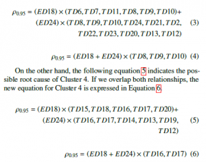
Figure 6: Rank Order Clustering – Cluster 1

ROC Pattern on four quadrant: Initial, Pre-Fault, Fault and Post-Fault for Cluster 1. The blue shaded region with red boxes represent the cluster of a high correlation value between 0.95 to 1.00.

Table 3: Summary of Sensitivity Index Description TD8 TD9 TD10 TD16 TD17 ED18 0.97919 0.97138 0.96878 0.98337 0.96881 ED24 0.95838 0.96982 0.996982 0.95842 0.97089

Combining Equation 4 with Equation 6, the sensitivity index is expressed in Table 3. With that, Event Modeller has reduced the dimensional to a smaller scale that will help the system engineer decide which relationship is liable to this fault. The following section will be discussed on the relationship between the observed data and the KPIs to validate the findings of the Event Modeller. Figure 6 and Figure 7 represent the pattern of the ROC system state for Cluster 1 and Cluster 4, respectively.

3.2.4       Relationship between the observed data against Key Performance Indicators

The KPIs are the translated index of the machine operation. It provides operational information for the decision-making of both the machine and the system operator. Four main KPIs have been adapted in this experiment known as Availability (A), Instantaneous Utilization (IU), Schedule Utilization (SU) and Performance (P). Having these four KPIs in line with CSU machine data, the possible root cause of frequent harmonic failure could be determined.

The following steps have been taken to analyze the data: (1) Select fault dataset from the Predictive Model Dataset. (2) Identify the fault observed data location. (3) Distinguish observed data according to Environment Variables, Electrical Variables and Motor Variables. (4) Plot Environment Variables data against KPIs. (5)

Plot Electrical Variables data against KPIs. (6) Plot Motor Variables data against KPIs.

The easiest way to identify fault events is by exploring the main incomer trip data. Theoretically, the entire electrical system will be tripped when there is a REGEN fault. Although it may conflict with other events in which the operator may trip the main incomer on purpose, the system could automatically distinguish between the actual fault and the simulated fault using the translated KPIs data.

For example, when a fault occurred during the operation, the data of the KPIs will hold the value in percentage. This verifies that the fault that occurred is genuine. If the machine is stopped or not operated, the value is either zero or hold to a specific value. In this example, the same dataset used in the previous experiment was chosen. This is to compare the relationship between the data observed using both techniques. The dataset dated 30^th January 2019 was therefore sampled between 12:47 pm and 13:03 pm. The target data was then divided into three and plotted against the KPIs as follows:

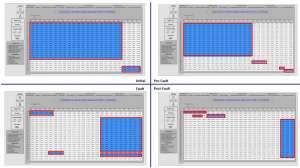
Figure 7: Rank Order Clustering – Cluster 4

ROC Pattern on four quadrant: Initial, Pre-Fault, Fault and Post-Fault for Cluster 4. The blue shaded region with red boxes represent the cluster of a high correlation value between 0.95 to 1.00.

Table 4: Summary of Electrical Variables Description ED1 ED2 ED4 Min 427.33 V 9.66 A 1.84 % Max 427.47 V 242.93 A 2.19 % Average 427.44 V 73.13 A 2.00 %

Figure 8 shows the observed electrical data against the KPIs when electrical faults occurred. This graph is quite revealing in several ways. First, the main fault has been observed. The chart reveals that the main fault occurred at 09:50. This is the turning point of all events. Next, the four KPIs are observed. The performance was initiated at 100% and remained for 1 minute. It was then exponentially reduced to 16% when the main fault occurred. This indicates that the unloading of coal has stopped immediately after 1 minute.

On the other hand, both Instantaneous Utilization and Schedule Utilization started at 58% and gradually decreased to 35% at 04:24.

At this point, Schedule Utilization bounces back to 39%, but Instantaneous Utilization remains reduced to 30% until the main fault event occurs. The availability started at 95% and remained until 04:24 before it gradually decreased when the main fault occurred. These trends have shown that there is a relationship between the main fault and the KPIs. Table 5 summarised the KPI results.

Moving to electrical variables, the main input voltage (ED1) remains at 427V for the entire time. Although the fault occurred, the main input voltage does not respond to this. This validates that the fault is not caused by power disturbances from the supply, such as transient, interruption, under-voltage or over-voltage. The Main Incomer Current (ED2) pattern was then observed. Before the fault, ED2 shows the current drawing of the electrical distribution. The pattern is based on loads of the motor during machine operation.

However, when the fault occurred, trends show that ED2 is responding to the event. An instantaneous drop was discovered during this period. ED2 does not fall to zero because the energy was still drawn from the maintenance feeder for essential loads. The main incoming THD (ED4) has also been observed. ED4 has been generated assuming that there will be no harmonic distortion during these events. The ED4 pattern remains at an average of 2.0% throughout the sampling time, indicating that the THD remains at IEEE 519 Standards. Table 4 summarised the electrical variables.

Meanwhile, to further explain the relationship between the motor variables and the KPIs, Figure 9 shows the current drawing of five main processes in the CSU machine. These include Bucket Elevator Current (ED17), Portal Conveyor Current (ED18), Travel Current (ED19), Boom Conveyor Current (ED20) and Hydraulic Power Pack (ED21). In order to validate the ED2 from the previous graph, this chart reveals that ED2 has a linear relationship with all motor variables within this graph. For example, when ED17 was drawn at the beginning of the sampling and all other motor loads were added during that period the ED2 measurement reached its peak value. Some attention is given to the small circle in the chart. It is clear that there was some instability happening at 01:48, which could be linked to the fault.

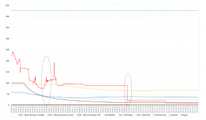
Figure 8: Electrical Variables vs KPIs

This figure illustrates the relationship between the Machine KPIs (Availability, Instantaneous Utilization, Schedule Utilization, and Performance) against the observed electrical data (Voltage, Current, Harmonic, Incomer and Regen) when the same event of electrical faults occurred at Time: 09:50.

Table 5: Summary of KPIs Description A IU SU P Min 64.37 % 25.01 % 34.82 % 11.52 % Max 91.67 % 58.33 % 58.33 % 100.00% Average 76.43 % 32.48 % 39.59 % 26.72 %

ED18 had an impulsive signal and remained zero after that event. On the other hand, ED19 has also revealed some dramatic changes. Just after ED18 had an impulsive signal, ED19 experienced some negative distortion for 12 seconds, followed by an interruption for 48 seconds and a further positive distortion for 60 seconds completely before it stopped. Another attention has to be made at ED17. In the beginning, ED17 had drawn some fluctuation current and had spiked for a few seconds before stopping at 00:40. The trend shows that ED17 is struggling to recover, but ends up stopping when the main fault has occurred. Otherwise, all other motor variables are operating in their normal state. Table 6 summarised the motor variables.

Figure 10 displays the environment data observed against the KPIs when the same electrical faults have occurred. Five environmental data were reported, including Panel Humidity (ED3), Panel Temperature (ED5), E-House Temperature (ED6), Wind Speed

(ED12) and E-House Humidity (ED24). Attention must be given to the humidity and temperature of the electrical room where the electrical distribution panel is located. The pattern has shown an instant increase of ED24 at 02:36. The humidity builds up and reaches its highest peak at 58% and slowly decreased with two spikes before the fault occurred. On the other hand, ED3 has also been increased but not as much as ED24. ED5 has an average temperature of 33.13 degrees Celsius, while ED5 has an average temperature of 17.82 degrees Celsius. Eventually, ED12 fluctuates within the normal range. Table 7 summarised the environment variables.

Figure 9: Motor Variables vs KPIs

3.2.5       Discussion

Table 6: Summary of Motor Variables Description ED17 ED18 ED19 ED20 ED21 Min 0.00 A -2.96 A -133.97 A 0.00 A 0.05 A Max 119.31 A 25.67 A 97.87 A 54.41 A 52.05 A Average 5.41 A 0.69 A 2.49 A 5.03 A 30.60 A

The main outcome of the experiment is to show how the proposed technique can be used as a tool to reduce the dimensions of a highly complex system. In this case study, 96 TDs were analyzed against 24 EDs in real-time to help system engineers visualize any changes to the system state. The EMDA implementation will group high correlation system parameters in the form of matrices and place them in mutually exclusive blocks. Having a huge matrix, however, will make things difficult. The matrix needs to be presented as a square for clear visibility. Thus, the 96 TDs were divided into 4 clusters, where each cluster has a relationship with 24 EDs. The example accessed a 16-minute dataset that belongs to a fault population. The result for each cluster was shown in a four-quadrant to show the pattern change. In this example, there is a significant change in the pattern observed in Cluster 1 and Cluster 4. Further analysis of the two clusters suggested a new formula representing the state of the system. After the fault event, the new formula for Cluster 1 and Cluster 4 is expressed in Equation 4 and Equation 6, respectively. As a result of these equations, the main culprit of the fault was identified. The ED variables were reduced from 24 EDs to 2 EDs (a decrease of 91.76%) while the TDs variable was reduced from 96TDs to 5TDs (a decrease of 94.79%). As listed in Table 3, the possible root causes of the fault are the combination of:

1. Portal Conveyor Current (ED18) with Rotary Feeding Table Motors (TD8), Bucket Elevator Motors (TD9), Bucket Elevator Brake Motors (TD10), Busy Rotary Table (TD16) and Busy Bucket Elevator (TD17) or
2. E-House Humidity (ED24) with Rotary Feeding Table Motors (TD8), Bucket Elevator Motors (TD9), Bucket Elevator Brake Motors (TD10), Busy Rotary Table (TD16) and Busy Bucket Elevator (TD17)

Further analysis with the KPIs will validate the existence of unknown events that could be linked to a harmonic problem. In normal circumstances, electrical variables such as voltage, current and THD should have a linear relationship with the KPIs. As the KPIs responded to the fault, the electrical variables should also respond. However, the voltage and the harmonic measurement remain constant after the fault has occurred. Although current measurements have responded to this fault, trends show that the current value is not zero. It indicates that there was still a current drawing for the essential loads. Therefore, this eliminates the possibility of machine failure due to electrical variables.

Moving to the motor variables, as explained in the result, ED17, ED18 and ED19 showed some undiscovered events that could lead to fault. When comparing the performance trend to ED17, the performance measurement falls in line with the activity of the bucket elevator. Although the trends for ED17 fluctuate before it stops, this could be explained from the perspective of uneven coal inside the bucket. On the other hand, ED18 has experienced an impulsive signal that leads to an immediate stop. However, looking at the timing of this event, it took about 9 minutes for the fault to happen. The same goes for ED19, which experienced negative and positive distortions right after ED18. This can be claimed as a result of an event. However, when it comes to the type of operation, ED19 is a travel motor that operates in two directions. Although some distorted measurements were made, this could be explained by the number of motors that were operating. There were ten motors in service working at different efficiency levels. Having said that, the motor variables are also excluded from being the root cause of the fault.

Figure 10: Environment Variables vs KPIs

Turning to environment variables, the trends in Figure 10 have shown some indications that the humidity could be related to the fault. The rise in humidity up to 58.06% shows that the state of the system has been compromised. Although high humidity patterns started 7 minutes before the fault, the measurement continuously retained above 40 % after the fault. This type of phenomena takes a fixed amount of time to reach the fault level. To explain this phenomenon, we take an example of preheating an oven. When a person decides to bake a cake, the oven needs to be heated to the right temperature before putting the cake inside the oven. Although it takes a few seconds to turn the oven on, it may take a few minutes to get the right temperature. This phenomenon is referred to as a fixed time delay deterministic event. However, if the person warms up the oven, without shutting the oven door, it may take longer to get to the right temperature. This phenomenon is referred to as a deterministic sequence of different input events. The heat produced in the oven was cooled by the amount of cold air present in the surroundings, which would delay the oven pre-heating process.

Table 7: Summary of Environment Variables Description ED3 ED5 ED6 ED12 ED24 Min 10.35 % 31.41 degC 17.12 degC 2.22 m/s 30.64 % Max 18.52 % 35.54 degC 18.16 degC 9.19 m/s 58.06 % Average 14.95 % 33.13 degC 17.82 degC 6.74 m/s 39.21 %

When we relate this to our case study, the power electronic component such as choke, rectifier, REGEN and control drives produce an excessive amount of heat during operation. To ensure that the heat is kept at certain limits, two units of air conditioners were designed to combat this heat. However, after considering the amount of heat generated in the room along with the hot and humid climate of Malaysia throughout the year, experts have reviewed and decided to install two additional air conditioners to cater for this amount of heat. As a result, when CSU machine is fully operational, the four-unit air conditioners are sufficient to cool down the electrical room. However, when the machine stops at intervals, the air conditioners are found oversized to the power electronic component. As a consequence, the humidity increases; the component becomes wet, resulting in machine failure. The humidity in the electrical switchgear room must be maintained at an elevated temperature relative to the ambient inside the room. Condensation is usually considered a problem only if the humidity in the switchgear room is 65% or greater [44]. Although the humidity in this example does not reach 65%, considering the machine has been running for a decade, the efficiency of the machine may decrease as the humidity may be the contributing factor. This finding suggests that there is a relationship between the humidity and the fault.

As mentioned earlier, this paper’s main outcome is to show how the EMDA can be used as a tool to reduce the dimensions of a highly complex system. 96 Triggered Data were scanned against 24 Event Data, which then formulated an equation representing the system state in a single second. This sort of like a ”scanner” that will keep converting a complex relationship into a simple equation (a huge reduction of dimensionality) in a low computational effort. The results in Table 3 shows that the complex relationship has been reduced to 2 EDs against 5 TDs. Further analysis with the KPIs has validated the existence of unknown events that linked to the frequent harmonic failure. The rise in humidity level shown in Figure 10 has proven that the system state has been compromised. In comparison, other variables such as electrical variables, motors and other environment do not show any evidence that compromises the system state. Besides, the relationship between the observed data and the KPIs appears to be consistent. The suggested finding was tested at site, and the operators confirmed the importance of humidity factor (environmental factor) in the machine’s performance. A humidity regulator has been suggested to be installed at the site. The control of the regulator was linked to the plant automatic control system.

4. Conclusions

Managing repetitive harmonic failures in an industrial application is a recursive, costly and time-consuming exercise. Industrial data are multidimensional and random in nature. The problem with analyzing this data is that many events do not necessarily repeat often enough to have statistical significance. Still, they cause minor or major faults and need to be captured and understood. Identical machines perform differently in different environments and conditions. In most cases, PQ engineers focus on the fundamental problem, transforming the power system signal into various signal processing methods to locate the fault. An Event Modeller technique, which is low in the computational effort, has been considered to solve this problem. This technique, which is extremely computational effective, managed to reduce system state definitions’ complexity into a simpler formulation. Also, the performance metrics translated from the machine operation are now automated and require minimum operator intervention. It reduces wrong interpretations and possible mistakes in decision making. However, one of the method’s weaknesses is its reliance on technical expert judgement on adjusting the threshold settings. One of the ongoing research endeavours of the authors is to automate the trigger detection phenomena.

In this present work, authors focused on reducing dimensionality while collectively including the modelling equation’s performance metrics parameter to verify the system state. Two approaches were taken to validate and verify the propose EMDA algorithm. First was the simulation process (SiL). It considered the voltage, humidity, harmonic, slewing movement, luffing movement, travelling movement, temperature, and wind speed as system output variables. Two types of triggering data, i.e. Static TD and Dynamic TD were considered. K-disturbance signal was generated for the five (excluding movements) output variables. The results show that, as the disturbance is induced, the sensitivity indices were reduced by an average of 8.2% for Static TD and 15.94% for Dynamic TD. However, when the disturbance was removed, the sensitivity indices regained by an average of 3.218% and 6.023% for Static TD and Dynamic TD consecutively. As a result, the Dynamic TD was chosen for the field experiments. In the field experiment (HiL), 914 data series in realtime were acquired from the SCADA. Each dataset is containing 96 Input vs 24 Output parameters. The results show that two new parameters were detected to significantly impact Harmonic Filters; humidity and portal conveyor current (velocity of the conveyor). The tests proved that humidity as an environmental factor is linked to the frequent harmonic problems. This revelation was also verified by looking up the historical evidence of humidity data against the frequency of failures and the variation in the feeder’s speed (conveyor). In the future, the proposed EMDA will be integrated as a vehicle for training supervised machine learning models to predict the remaining useful life of the filter as a predictive

Acknowledgement

This work has received financial support from Malaysia’s government sponsorship, MARA. The authors would like to acknowledge the editor and anonymous referees. The use of existing shop-floor in modern manufacturing to measure and monitor industrial KPIs has been a trend. In [38], the author used Object Linking and Embedding (OLE) which integrates with Discrete Event Simulation (DES) modelling capabilities to measure

1. F. Z. M. Fadzil, A. Mousavi, M. Danishvar, “Simulation of Event-Based Tech- nique for Harmonic Failures,” in 2019 IEEE/SICE International Symposium on System Integration (SII), 66–72, IEEE, 2019, doi:10.1109/SII.2019.8700381.
2. U. Singh, S. N. Singh, “Application of fractional Fourier transform for classifi- cation of power quality disturbances,” IET Science, Measurement & Technol- ogy, 11(1), 67–76, 2017, doi:10.1049/iet-smt.2016.0194.
3. M. Panteli, P. Mancarella, “Influence of extreme weather and climate change on the resilience of power systems: Impacts and possible mitigation strategies,” Electric Power Systems Research, 127, 259–270, 2015, doi:10.1016/j.epsr. 2015.06.012.
4. M. K. Saini, R. Kapoor, “Classification of power quality events–a review,” International Journal of Electrical Power & Energy Systems, 43(1), 11–19, 2012, doi:10.1016/j.ijepes.2012.04.045.
5. Z. Huang, M. Li, A. Mousavi, M. Danishva, Z. Wang, “EGEP: An Event Tracker Enhanced Gene Expression Programming for Data Driven System En- gineering Problems,” IEEE Transactions on Emerging Topics in Computational Intelligence, 3(2), 117–126, 2019, doi:10.1109/TETCI.2018.2864724.
6. M. Morcos, W. A. Ibrahim, “Electric Power Quality and Artificial Intellignece: Overview and Applicability,” IEEE Power engineering review, 19(6), 5–10, 1999, doi:10.1109/MPER.1999.768508.
7. D. Saxena, K. Verma, S. Singh, “Power quality event classification: an overview and key issues,” International Journal of Engineering, Science and Technology, 2(3), 186–199, 2010.
8. D.C. Robertson, O. I. Camps, J. S. Mayer, W. B. Gish, “Wavelets and elec- tromagnetic power system transients,” IEEE Transactions on Power Delivery, 11(2), 1050–1058, 1996, doi:10.1109/61.489367.
9. S. Santoso, E. J. Powers, W. M. Grady, P. Hofmann, “Power quality assessment via wavelet transform analysis,” IEEE transactions on Power Delivery, 11(2), 924–930, 1996, doi:10.1109/61.489353.
10. J. Barros, R. I. Diego, “Analysis of harmonics in power systems using the wavelet-packet transform,” IEEE Transactions on Instrumentation and Mea- surement, 57(1), 63–69, 2008, doi:10.1109/TIM.2007.910101.
11. S. Shukla, S. Mishra, B. Singh, “Empirical-mode decomposition with Hilbert transform for power-quality assessment,” IEEE transactions on power delivery, 24(4), 2159–2165, 2009, doi:10.1109/TPWRD.2009.2028792.
12. R. G. Stockwell, “A basis for efficient representation of the S-transform,” Digi- tal Signal Processing, 17(1), 371–393, 2007, doi:10.1016/j.dsp.2006.04.006.
13. S.H. Cho, G. Jang, S.-H. Kwon, “Time-frequency analysis of power-quality disturbances via the Gabor–Wigner transform,” IEEE transactions on power delivery, 25(1), 494–499, 2010, doi:10.1109/TPWRD.2009.2034832.
14. C. Norman, J. Y. Chan, W. H. Lau, L. L. Lai, “Hybrid Wavelet and Hilbert Transform With Frequency-Shifting Decomposition for Power Quality Analy- sis.” IEEE Trans. Instrumentation and Measurement, 61(12), 3225–3233, 2012, doi:10.1109/TIM.2012.2211474.
15. B. Biswal, P. K. Dash, S. Mishra, “A hybrid ant colony optimization technique for power signal pattern classification,” Expert Systems with Applications, 38(5), 6368–6375, 2011, doi:10.1016/j.eswa.2010.11.102.
16. K. Manimala, K. Selvi, R. Ahila, “Optimization techniques for improving power quality data mining using wavelet packet based support vector machine,” Neurocomputing, 77(1), 36–47, 2012, doi:10.1016/j.neucom.2011.08.010.
17. R. Ahila, V. Sadasivam, K. Manimala, “An integrated PSO for parameter de- termination and feature selection of ELM and its application in classification of power system disturbances,” Applied Soft Computing, 32, 23–37, 2015, doi:10.1016/j.asoc.2015.03.036.
18. C. Cortes, V. Vapnik, “Support-vector networks,” Machine learning, 20(3), 273–297, 1995, doi:10.1007/BF00994018.
19. L. A. Zadeh, “Fuzzy sets,” in Fuzzy Sets, Fuzzy Logic, And Fuzzy Systems: Selected Papers by Lotfi A Zadeh, 394–432, World Scientific, 1996.
20. S. Khokhar, A. A. M. Zin, A. S. Mokhtar, N. A. M. Ismail, N. Zareen, “Auto- matic classification of power quality disturbances: A review,” in 2013 IEEE Student Conference on Research and Developement, 427–432, 2013, doi: 10.1109/SCOReD.2013.7002625.
21. D. Granados-Lieberman, R. Romero-Troncoso, R. Osornio-Rios, A. Garcia- Perez, E. Cabal-Yepez, “Techniques and methodologies for power qual- ity analysis and disturbances classification in power systems: a review,” IET Generation, Transmission & Distribution, 5(4), 519–529, 2011, doi: 10.1049/iet-gtd.2010.0466.
22. M. McGranaghan, “Overview of Power Quality Standards,” PQ Network Inter- net Site, http://www. pqnet. electrotek. com/pqnet, 1998.
23. I.W. Group, et al., “IEEE Recommended Practices and Requirements for Harmonic Control in Electrical Power Systems,” IEEE STD, 519–1992, 1992.
24. B. IEC, “61000-3-4,” Electromagnetic compatibility (EMC)-part, 3–4, 1998.
25. P. Muchiri, L. Pintelon, “Performance measurement using overall equipment effectiveness (OEE): literature review and practical application discussion,” International journal of production research, 46(13), 3517–3535, 2008, doi: 10.1080/00207540601142645.
26. V. C. Angadi, A. Mousavi, D. Bartolome´, M. Tellarini, M. Fazziani, “Re- gressive Event-Tracker: A Causal Prediction Modelling of Degradation in High Speed Manufacturing,” Procedia Manufacturing, 51, 1567–1572, 2020, doi:10.1016/j.promfg.2020.10.218.
27. V. C. Angadi, A. Mousavi, D. Bartolome´, M. Tellarini, M. Fazziani, “Causal Modelling for Predicting Machine Tools Degradation in High Speed Produc- tion Process,” IFAC-PapersOnLine, 53(3), 271–275, 2020, doi:10.1016/j.ifacol. 2020.11.044.
28. M. Danishvar, V. C. Angadi, A. Mousavi, “A PdM Framework Through the Event-based Genomics of Machine Breakdown,” in 2020 Asia-Pacific Inter- national Symposium on Advanced Reliability and Maintenance Modeling (APARM), 1–6, IEEE, 2020, doi:10.1109/APARM49247.2020.9209530.
29. Z. Huang, V. C. Angadi, M. Danishvar, A. Mousavi, M. Li, “Zero Defect Man- ufacturing of Microsemiconductors–An Application of Machine Learning and Artificial Intelligence,” in 2018 5th International Conference on Systems and Informatics (ICSAI), 449–454, IEEE, 2018, doi:10.1109/ICSAI.2018.8599292.
30. M. Danishvar, V. Vasilaki, Z. Huang, E. Katsou, A. Mousavi, “Application of Data Driven techniques to Predict N 2 O Emission in Full-scale WWTPs,” in 2018 IEEE 16th International Conference on Industrial Informatics (INDIN), 993–997, IEEE, 2018, doi:10.1109/INDIN.2018.8472075.
31. M. Danishvar, A. Mousavi, P. Broomhead, “EventiC: A Real-Time Unbiased Event-Based Learning Technique for Complex Systems,” IEEE Transactions on Systems, Man, and Cybernetics: Systems, 2018, doi:10.1109/TSMC.2017. 2775666.
32. S. Tavakoli, A. Mousavi, S. Poslad, “Input variable selection in time-critical knowledge integration applications: A review, analysis, and recommenda- tion paper,” Advanced Engineering Informatics, 27(4), 519–536, 2013, doi: 10.1016/j.aei.2013.06.002.
33. M. Danishvar, A. Mousavi, P. Sousa, “EventClustering for improved real time input variable selection and data modelling,” in 2014 IEEE Conference on Con- trol Applications (CCA), 1801–1806, 2014, doi:10.1109/CCA.2014.6981574.
34. S. Tavakoli, A. Mousavi, P. Broomhead, “Event tracking for real-time unaware sensitivity analysis (EventTracker),” IEEE Transactions on Knowledge and Data Engineering, 25(2), 348–359, 2013, doi:10.1109/TKDE.2011.240.
35. J. R. King, “Machine-component grouping in production flow analysis: an approach using a rank order clustering algorithm,” International Journal of Pro- duction Research, 18(2), 213–232, 1980, doi:10.1080/00207548008919662.
36. M. R. Kumar, G. P. Rao, “Design and implementation of 32 bit high level Wallace tree multiplier,” Int. Journ. of Technical Research and Application, 1, 86–90, 2013.
37. A. Mousavi, H. Siervo, “Automatic translation of plant data into management performance metrics: a case for real-time and predictive production control,” International Journal of Production Research, 55(17), 4862–4877, 2017, doi: 10.1080/00207543.2016.1265682.
38. S. X. Ding, S. Yin, K. Peng, H. Hao, B. Shen, “A novel scheme for key per- formance indicator prediction and diagnosis with application to an industrial hot strip mill,” IEEE Transactions on Industrial Informatics, 9(4), 2239–2247, 2012, doi:10.1109/TII.2012.2214394.
39. K. Ragunathan, S. Ravindranathan, S. Naveen, “Statistical KPIs in HMI panels,” in 2015 International Conference on Green Computing and Internet of Things (ICGCIoT), 838–843, IEEE, 2015, doi:10.1109/ICGCIoT.2015.7380579.
40. N. Kang, C. Zhao, J. Li, J. A. Horst, “Analysis of key operation performance data in manufacturing systems,” in 2015 IEEE International Conference on Big Data (Big Data), 2767–2770, IEEE, 2015, doi:10.1109/BigData.2015.7364078.
41. G. UK, “Greenhouse Gas Reporting: Conversion Factors 2017,” GOV. UK [Online]. Available: https://www. gov. uk/government/publications/greenhouse- gas-reporting-conversion-factors-2017., 2017.
42. Y. Zhu, ”Multivariable system identification for process control”, Elsevier, 2001.
43. J. E. Bowen, M. C. Moore, M. W. Wactor, “Application of switchgear in unusual environments,” in 2010 Record of Conference Papers Industry Applications Society 57th Annual Petroleum and Chemical Industry Conference (PCIC), 1–10, IEEE, 2010, doi:10.1109/PCIC.2010.5666870.

(Click Here)