1. Introduction

With the development of industry and technology, various industrial rotating machines have become capable of handling high speeds and heavy loads, which cause massive mechanical and thermal loads, resulting in their breakdown [1]. When a rotating machine fails, fault diagnosis is very important as time and economic loss can occur. Therefore, a countermeasure is required to check the condition of rotating machines and to diagnose faults. According to statistical data, 45%–55% of failures in rotating machines are due to faults in the bearings [2]. Monitoring the condition of the rotating machine to detect its faults helps reduce losses [3]-[5].

Machine learning algorithm is a common method of diagnosing faults of rotating machines.

In general, the fault diagnosis method of rotating machines using a machine learning algorithm is divided into four steps: (1) data acquisition, (2) feature extraction, (3) machine learning algorithm training (neural network training), and (4) classification [6]-[9].

The data acquisition step is the process of obtaining a signal that indicates the state of a rotating machine using a sensor. A noise-measuring device, the electric current signals of the motor, and vibration signals are used to obtain signs that indicate the state of the rotating machine [10]-[12]. Among them, the commonly used method detects the fault of the rotating machine by obtaining vibration signal data that are the easiest to measure and can clearly indicate the state of the rotating machine [13].

In the feature extraction step, signs that indicate the state of the rotating machine are extracted from the vibration signals. In general, a signal measured from the rotating machine consists of a mixture of noise and a sign indicating the state of the rotating machine. If vibration signals containing noise are used as input values in the machine learning algorithm, it is difficult to accurately diagnose the state of the rotating machine due to the noise. Hence, noise should be removed from the vibration signals through feature extraction to use them as input values for the machine learning model.

The most common feature extraction methods use filters and signal decomposition [14]-[16]. The widely used methods of diagnosing faults in vibration signals include empirical mode decomposition (EMD) technique, which uses intrinsic mode function (IMF) to decompose the signals, and wavelet transform method, which uses the wavelet function to decompose the signals.

The EMD technique yields outstanding performance when detecting faults of rotating machines [17]. However, it requires to combine sub-band signals because the sub-bands decomposed by IMF are generally not orthogonal to each other [18].

The wavelet transform method has the advantage of adjusting the cycle and amplitude to show the features more clearly in the vibration signals of rotating machine and to remove the noise included in the vibration signals [19], [20].

In the machine learning algorithm training step, the algorithm is trained by using the features extracted from the vibration signals as input values for the machine learning algorithm. Among the various machine learning algorithms, the algorithms using deep learning show better performance, and among the deep learning algorithms, convolution neural network (CNN) shows superior performance.

In the classification step, the test data, which are not used in the training step, are used to classify the state of the rotating machine, and the indicator showing the performance of the model can be derived.

Eren used CNN to diagnose faults of rotating machines but diagnosed their faults based solely on the performance of the CNN model without considering the method of removing the noises [21]. Meanwhile, Yuan used discrete wavelet transform and CNN to improve the performance of the existing rotating machine fault diagnosis model. However, there was a limitation in showing the suitable performance in a poor environment where noise can be measured substantially because the experiment was conducted without reflecting noise [22].

In this study, we used continuous wavelet transform method, to decompose vibration signals into noise, and signals indicating the state of the rotating machine to detect its faults, and extracted signals that can be used to detect the faults of the rotating machine, from the decomposed signals. The extracted features were used as input values of CNN, a deep-learning technique, to classify the faulty state of the rotating machine. Furthermore, we added white Gaussian noise to investigate the effectiveness of the corresponding algorithm through performance comparison between the model and conventional machine learning methods in a poor environment where a large amount of noise can be observed.

2. Theory

2.1. Continuous wavelet transform

The advantage of the wavelet transform method is that the wavelet function with dynamic resolution can be used to efficiently analyze the vibration signals, unlike Fourier transform, which cannot accurately display the characteristics of non-cyclic signals due to the fixed resolution [23][24]. The time series analysis using the wavelet transform is defined as follows.

In Eq. (1), the signal is decomposed by shifting the wavelet function to the time axis by  and scaling by a. If the mother wavelet is given, then continuous wavelet transform (CWT) of the signal f(t) is defined by Eq. (2).

The wavelet coefficient obtained in Eq. (2) indicates the similarity between f(t) and . The wavelet transform produces the decomposition of the time scale of f(t), but the time-frequency region can be obtained by the pseudo-frequencies.

The relationship between the scale and the pseudo-frequencies changes depending on the center of the wavelet function, performance of the scale, and sampling cycle and maximizes the spectrum of the wavelet function with the given scale. The relationship of these parameters is expressed by Eq. (3).

In Eq. (3),  denotes the center frequency,  is the sampling cycle, and  shows the result of the pseudo-frequency. The entire signal is synthesized by applying the inverse continuous wavelet transform (ICWT) defined in Eq. (4) as follows:

here,  is the acceptance constant obtained when the mother wavelet satisfies all requirements.

2.2. Convolutional Neural Network

CNN was inspired by the principle of recognizing objects in the visual cortex of the brain and was derived from the field of deep learning. It consists of convolutional layer, pooling layer, and fully connected layer [25].

The main function of a convolutional layer is to obtain a feature map through the convolutional operation of filter for the input. The convolutional layer typically consists of learnable kernel and bias. The size of the kernel corresponds to the size of the filter, and the depth of the kernel corresponds to the number of channels in the feature map. The input of the convolutional layer can be calculated by the weight and the inner product of cognitive region, as expressed by Eq. (5).

      In Eq. (5),  refers to the convolutional value of ith channel in the convolutional layer l,  refers to the ith output of the pooling layer l-1,  refers to the kernel of the convolutional layer l,  refers to the bias of the jth channel in the convolutional layer l, and * refers to the convolutional operation.

      After the convolutional operation is completed, the value of convolutional layer is calculated according to the activation function. The role of the activation function is to perform the nonlinear projection for the input of the neuron. Rectified linear unit (ReLU), one of activation functions, is used for pattern recognition. The ReLU function shows excellent performance in accelerating convergence and solving vanishing gradient problems. Therefore, the ReLU is used as the activation function of a convolutional layer, and the output of convolutional layer 1 can be expressed by Eq. (6).

Here,  represents the output of the jth channel in the convolutional layer l, and ( ) refers to the activation function.

      After the convolutional layer operation, the pooling layer is used to extract additional features. It plays a role of reducing the dimensions of the output of the previous layer. Therefore, the key purpose of this layer is to reduce the volume of data to reduce the computation time on the computer. Types of pooling layer include max pooling, average pooling, logarithmic pooling, and weight pooling.

      Max pooling is used to classify operation because it can speed up the convergence and improve the generalization. Max pooling function can be expressed by Eq. (7).

       represents the window of the pooling layer that can shift to a certain step, and  correspond to the dimensions of the pooling layer. Further,  refers to the output of jth channel in the convolutional layer, and  refers to the overlap between the pooling layer and the channel’s output.

      In general, the CNN model contains multiple convolutional and pooling layers and extracts feature maps sequentially. The extracted feature map is transformed into a vector, which is used as an input of a fully connected layer. The main function of the fully connected layer is to extract additional features and connect the output step to the softmax classifier. A fully connected layer usually consists of 2 or 3 hidden layers, and all neurons of a hidden layer can be shown by Eq. (8).

       refers to the weight matrix of the fully connected layer,  represents the bias, and  represents the activation function of the fully connected function.

2.3. Batch normalization

In general, as the depth of the neural network structure increases, the distribution of features changes, and the overall distribution gradually approaches both ends of the nonlinear function value interval. This phenomenon is called gradient diffusion, which causes a problem with the convergence of the model. To resolve this problem, the Google DeepMind team proposed batch normalization technique in 2014 [26].

The key purpose of the batch normalization technique is to revert the distribution of all neurons to the standard normal distribution through a specific normalization method. Batch normalization can re-parameterize almost all neural networks and, thus, can be used for any hidden layer. Batch normalization, which optimizes neural networks, can improve the performance of neural networks, such as faster convergence, faster learning time, ability to allow higher learning rate, and easier initialization of weights.

First, normalization can make each scalar feature with the mean 0 and the unit variance, as expressed in Eq. (9).

However, if Eq. (9) is used to directly normalize the features of a certain layer, the learned features can be affected, thereby reducing the performance of the neural network. To overcome this problem, each normalized  is modified based on two adjustment parameters,  and , aiming at scaling and shifting the normalized values. This process can be expressed by Eq. (10).

here,  and  are parameters that can be used to learn the method of recovering the characteristic distribution of the existing neural network. By setting  and , the existing activation can be restored. In this case, the activation values are stably distributed during learning.

Second, because the mini-batch technique is used in training process, the specific activation  that possesses the B value in the mini-batch is , and the corresponding transformation is . Therefore, the batch normalization transform →  can be represented by Eqs. (11), (12), (13), and (14).

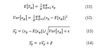here,  is a constant and is used to avoid undefined gradient values.

3. Experiment setup

This study required constructing a variety of dataset to enhance the accuracy of the fault detection of the rotating machine. Thus, we utilized the Case Western Reserve University Bearing Fault Database, which is widely used for fault detection of conventional rotating machines [27]. Because various researchers have conducted experiments using this database, there are several advantages: the data are reliable, and the performance comparison can be conducted with other learning algorithms. As shown in Figure 2, the test bench consists of a motor on the left, a torque transducer/encoder on the center, and a dynamometer on the right.

The vibration signals were measured in a total of four types: normal, ball fault, inner race fault, and outer race fault. The levels of crack consisted of 0.007, 0.014, and 0.021 inch, and the levels of load consisted of 0 HP, 1 HP, 2 HP, and 3 HP.

Figure 1 shows the fault detection process of rotating machine using vibration signals. Data having cracks of 0.007 inch were used, and the dataset was classified into Case 1 (0 HP), Case 2 (1 HP), Case 3 (2 HP), and Case 4 (3 HP), depending on the level of load. Each case consisted of 4,368 data: 1,092 for normal data, 1,092 for ball faults, 1,092 for inner race faults, and 1,092 for outer race faults. In addition, white Gaussian noise was increased in the vibration signals having cracks of 0.007 inch to verify the robustness to noise by CWT. As shown in Figure 3, the sample data were constructed to train the CNN model by performing the segmentation with 4,392 signals where white Gaussian noise was added in the actual vibration signals. For each sample data, continuous wavelet functions, such as morse, morlet, and bump wavelet, were applied, and CWT was used. The conversion to images with the size of 224 × 224 was performed to use them as inputs of CNN after signal preprocessing, as shown in Figure 2.

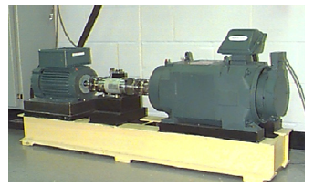Figure 1: Experiment setup

The CNN was constructed with 8 3 × 3 filters for the first layer of the CNN model, 16 3 × 3 filters for the second layer, and 32 3 × 3 filters for the third layer. Additional features were extracted through the fully connected layer, and the faults of rotating machine were classified using the softmax classifier. After the convolutional operation was completed in each layer, batch normalization and max pooling, a type of pooling layer, were applied.

To conduct the training of the constructed CNN model, 70% of 4,368 data in the entire dataset were used for the training process of the CNN model, and the rest were used to validate the trained CNN model. To validate the performance of the trained model, comparative analysis was performed with the DNN technique, a conventional vibration signal analysis method using artificial neural network (ANN).

Figure 2: Representation of proposed fault diagnosis structure

4. Simulation

As shown in Fig 3, CWT was performed through the continuous wavelet functions—namely, morse, morlet, and bump wavelet—using the white Gaussian noise-added vibration signals, and the results were used as input values of the CNN model.

To compare the performance of the generated CNN model, comparative analysis was performed using the ANN model by extracting statistical parameters, such as peak, entropy, skewness,
kurtosis, variance, and rms, and using them as the input values of the ANN, as shown in Figure 4.

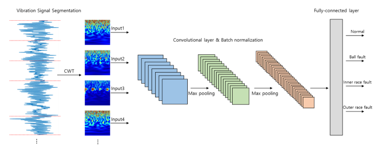Figure 3: The process of fault diagnosis in vibration signal using CWT & CNN.

Figure 4: Result of fault diagnosis (accuracy & loss) – (a) Case1(=0HP), (b) Case2(=1HP), (c) Case3(=2HP), (d) Case4(=3HP)

To compare the performance of the CNN model and the CWT for noise removal, we compared the accuracy and loss for each signal-to-noise ratio (SNR) level with those of the existing method, in which the parameters are extracted from the vibration signals and then used as inputs of the ANN, as shown in Figure 4.

When the SNR was 1 dB in the Case 1 (0 HP) dataset, the accuracy of the CNN model using morlet wavelet was 95.31% with a loss of 0.05869, that of the CNN model using bump wavelet was 90.25% with a loss of 0.11, and that of CNN model using morse wavelet was 90.13% with a loss of 0.124. Therefore, the performance was excellent compared to that of the ANN model. Furthermore, when the SNR level was reduced step by step, the CNN model using CWT showed that the accuracy converged to 100% at the SNR level of 8 dB, whereas the ANN model showed that the accuracy converged to 100% when the SNR level was 15 because of performance degradation in the denoising function.

In terms of loss, the CNN model using CWT showed the convergence close to 0 when the SNR level was 11 dB. However, the model using the ANN showed the convergence to 0 when the SNR level was 18 dB, indicating that the performance was lower than that of the CNN model.

When SNR was 1 dB in the Case2 (1 HP) dataset, the accuracy of the CNN model using morlet wavelet was 72.82% with a loss of 0.6254, that of the CNN model using bump wavelet was 86.12% with a loss of 0.3602, and that of the CNN model using morse wavelet was 86.09% with a loss of 0.3597. The differences were not large compared to those of the ANN model (accuracy: 71.7% and loss: 0.1388). When the SNR level was reduced, the accuracy converged to 100% at the SNR level of 10 dB in the CNN model using CWT. Conversely, the accuracy converged to 100% when the SNR level became 14 dB in the ANN model. Furthermore, in terms of loss, the CNN model using CWT showed the convergence to 0 when the SNR level was 10 dB, whereas the ANN model showed the convergence to 0 when the SNR level was 14 dB.

When the SNR level was 1 dB in the Case 3 (2 HP) dataset, the accuracy of the CNN model using morlet wavelet was 87.04% with a loss of 0.31, that of the CNN model using bump wavelet was 86.72% with a loss of 0.409, and that of the CNN model using morse wavelet 86.61% with a loss of 0.1232. Therefore, the performance was excellent compared to that of the ANN model (accuracy: 71.9% and loss: 0.1432).

When the SNR level was 1 dB in the Case 4 (3 HP) dataset, the accuracy of the CNN model using morlet wavelet was 85.13% with a loss of 0.2947, that of the CNN model using bump wavelet was 83.37% with a loss of 0.34924, and that of the CNN model using morse wavelet was 85.03% with a loss of 0.4238. Meanwhile, the accuracy and loss of the ANN model were 69.3% and 0.1431, respectively. As the noise signal decreased, the CNN model using CWT showed that the accuracy and the loss converged to 100% and 0, respectively, when the SNR level was 10 dB. However, the ANN model showed that the accuracy converged to 100% when the SNR level was 14 dB, and the loss converged to 0 when the SNR level was 16 dB. Based on these results of the vibration signal analysis, we have confirmed that the CNN model using CWT is more robust to noise than the existing method. Furthermore, we used the pooling layer and batch normalization to reduce the training time of the CNN model and improve the performance, thereby confirming the effectiveness and stability of the method, in comparison with the conventional signal analysis method.

5. Conclusion

In this study, vibration signal analysis was conducted to diagnose faults of rotating machines. Furthermore, to investigate the performance in actual work site environment, we conducted vibration signal analysis. Hence, we added white Gaussian noise in the vibration signals step by step and applied CWT. Subsequently, we extracted the images to use them as input values of the CNN. When we added the white noise from 1dB to 20dB to vibration signal, the proposed method converged to 100% accuracy from 8dB at no load, at 10dB at presence of load. The analysis results confirmed that CWT-applied CNN model showed superior performance compared to the existing signal analysis method.

6. Acknowledgment

This work was supported by the Technology Innovation Program (or Industrial Strategic Technology Development Program) (Grant number: No.20010132, development of the systematization platform for expending the industry of xEV parts) and 2019 Industrial Employment Crisis Area Technology (Grant number: P075100005, ESS Safety certification system for ships and international testing laboratory) funded By the Ministry of Trade, Industry & Energy(MOTIE, Korea).

1. A. H. Bonnett, G. C. Soukup, “Cause and analysis of stator and rotor failures in three-phase squirrel-cage induction motors”, IEEE Transaction on Industry Applications, 28(4), 921-937, 1992, 10.1109/PAPCON.1991.239667
2. Nandi, S., Toliyat, H. A., & Li, X., “Condition monitoring and fault diagnosis of electrical motors – a review”, IEEE Transactions on Instrumentation and Measurement, 65(11), 2646-2656, 2005, 10.1109/CMD.2008.4580260
3. B. Dolenc, P. Boskoski, D.Juricic , “Distributed bearing fault diagnosis based on vibration analysis”, Mech. Syst. Signal Process, 66-67, 521-532, 2016, https://doi.org/10.1016/j.ymssp.2015.06.007
4. L. Barbini, A.J. Hillis, J.L. du Bois, “Amplitude-cyclic frequency decomposition of vibration signals for bearing fault diagnosis based on phase editing”, Mech. Syst. Signal Process, 103, 76-88, 2018, https://doi.org/10.1016/j.ymssp.2017.09.044
5. E. EI-Thalji, Jantunen, “A summary of fault modeling and predictive health monitoring of rolling bearings”, Mech. Syst. Signal Process, 60-61, 252-272, 2015, https://doi.org/10.1016/j.ymssp.2015.02.008
6. W.K. Xi, Z.X. Li, Z. Tian, et al., “A feature extraction and visualization method for fault detection of marine diesel engines”, Measurement, 116, 429-437, 2018, https://doi.org/10.1016/j.measurement.2017.11.035
7. J.B. Yu, J.X Lv, “Weak fault feature extraction of rolling bearings using local mean decomposition-based multilayer hybrid denoising”, IEEE Trans. Instrum. Meas., 66(12), 3148-3159, 2017, 10.1109/TIM.2017.2751878
8. M. Amar, I. Gondal, C. Wilson, “Vibration spectrum imaging: a novel bearing fault classification approach”, IEEE Trans Ind. Electron., 51(1), 494-502, 2015, 10.1109/TIE.2014.2327555
9. B. Madahian, L.Y. Deng, R. Homayouni, “Development of a literature informed Bayesian machine learning method for feature extraction and classification”, BMC Bioinform, 16. , 2015, https://doi.org/10.1186/1471-2105-16-S15-P9
10. Chacon, J.L.F., Kappatos, V., Balachandran, W., & Gan, T.-H., 2015 “A novel approach for incipient defect detection in rolling bearings using acoustic emission technique”, Applied Acoustics, 89, 88-100., 2015, https://doi.org/10.1016/j.apacoust.2014.09.002
11. S. Singh, Kumar, A., & Kumar, N., ” Motor current signature analysis for bearing fault detection in mechanical system”, Procedia Materials Science, 6, 171-177, 2014, https://doi.org/10.1016/j.mspro.2014.07.021
12. J. Zarei, Tajeddini, M. A., & Karimi, H. R., “Vibration analysis for bearing fault detection and classification using an intelligent filter”, Mechatronics, 24(20), 151-157, 2014, https://doi.org/10.1016/j.mechatronics.2014.01.003
13. Kharche, P., P., & Ksgirsagar, S. V., “Review of fault detection in rolling element bearing”, International Journal of Innovative Research in Advanced Engineering, 1(5), 169-174, 2014, https://ijirae.com/images/downloads/vol1issue5/JNME10092(33).pdf
14. W. He. Z.N. Jiang., K. Feng, “Bearing fault detection based on optimal wavelet filter and sparse code shrinkage”, Measurement, 42(7), 1092-1102. 2009, https://doi.org/10.1016/j.measurement.2009.04.001
15. X. L. An, H. T. Zeng, W. W. Yang, et al., 2017, “Fault diagnosis of a wind turbine rolling bearing using adaptive local iterative filtering and singular value decomposition”, T. I. Meas. Control., 39(11), 1643-1648, 2017, https://doi.org/10.1177/0142331216644041
16. X. An, Weiwei Yang, Xuemin An, “Vibration signal analysis of a hydropower unit based on adaptive local iterative filtering”, P. I. Mech. Eng. C-J Mec. 231(7), 1339-1353, 2017, https://doi.org/10.1177/0954406216656020
17. Y. Li, M. Xu, X. Liang, “Huang Application of bandwidth EMD and adaptive multiscale morphology analysis for incipient fault diagnosis of rolling bearings”, IEEE Trans. Ind. Electron., 61(8), 6506-6517, 2017, 10.1109/TIE.2017.2650873
18. J.P. Yang, P.Z. Li, Yang, et al., “An improved EMD method for modal identification and a combined static-dynamic method fir damage detection”, Sound Vib., 240, 242-260, 2018, https://doi.org/10.1155/2014/317954
19. Q.B. He, “Vibration signal classification by wavelet packet energy flow manifold learning”, J. Sound Vib., 332(7), 1881-1894, 2013, https://doi.org/10.1016/j.jsv.2012.11.006
20. Q. Pan, L. Zhang, G. Dai, H. zhang, “Two denoising methods by wavelet transform”, IEEE Trans. Signal Processing, 47(12), 3401-3406, 1991, https://doi.org/10.1109/78.806084
21. Eren L., “Bearing Fault Detection by One-Dimensional Convoltional Neural Networks”, Mathematical Problems in Engineering, https://doi.org/10.1155/2017/8617315
22. Yuan Xie, Tao Zhang, “Feature Based on DWT and CNN for Rotating Machinery Fault Diagnosis”, IEEE Trans. CCDC, 29, 3861-3866, 2017 10.1109/CCDC.2017.7979176
23. V. Pichot, J.M. Gaspoz, S. Molliex, A. Antoniadis, Wavelet transform to quantify heart rate variability and to assess its instantaneous changes, J. Appl. Physiol.86(3), 1081–1091, 1991, http://dx.doi.org/10.1152/jappl.1999.86.3.1081
24. L.G. Gamero, J. Vila, F. Palacios, Wavelet transform analysis of heart rate variability during myocardial ischaemia, Med. Biol. Eng. Comput. 40, 72–78, 2002, http://dx.doi.org/10.1007/BF02347698.
25. X. Li, W. Zhang, Deep learning-based remaining useful life estimation of bearings using multi-scale feature extraction, Reliab. Eng. Syst. Saf. 182 208–218, 2019, http://dx.doi.org/10.1016/j.ress.2018.11.011.
26. J. Wang, S. Li, B. Han, et al., Construction of a batch-normalized autoencoder network and its application in mechanical intelligent fault diagnosis, Meas. Sci. Technol. 30, 1–14, 2019, http://dx.doi.org/10.1088/1361-6501/aaf319.
27. K.A. Loparo, “Bearing fault diagnosis based on wavelet transform and fuzzy inference”, Mechanical System and Signal Processing, 2005, https://doi.org/10.1016/S0888-3270(03)00077-3

(Click Here)

No. of Downloads Per Month

No. of Downloads Per Country