1. Introduction

Music is one of the most popular entertainments. There are 1.15 trillion users who stream video and audio-based music on digital platforms in 2019 and increased by 29.3% from the previous year. The increasing number of users are based on the fact that music could control people’s emotions, moods, or physiological arousal [1]. Besides users, music content also increases a lot every year. Large numbers of music content are making it hard for people to search relevant music, especially when it is unorganized. Therefore, there is a need to organize all music content, but it is very time consuming to do manually. In order to simplify this process, some music applications like Spotify and Youtube Music implement recommendation mechanisms or systems [2]. This recommendation system can suggest a list of relevant music from the library and becoming popular nowadays and crucial to prevent their customer to move on to another service [3].

Recommendation systems use two main approaches, content based and collaborative filtering (CF). Content based approach focuses on item metadata or attributes. For example, a music described by genre, singer, producer, etc. Otherwise, CF approaches focus on user preferences and are called as personalized recommendation systems. This approach analyzes the relationship between user and item. Similar users tend to be interested in similar items. User similarity can be measured by their history or review. Afterwards, user-item relation is used to predict what item might be liked by other users similar to him. Suggested items may vary for each user, due to different interests. Thus, CF approach has become popular and widely used in recommending items [4].

In CF, matrix factorization (MF) becomes one of the most popular techniques besides neighbour-based using similarity metric. Unfortunately, MF performance impeded due to inadequately capturing an advanced structure of user interaction data. Thus, it is required to develop another technique by using MF approach to obtain better results [5]. Recommendation system nowadays widely implements hybrid techniques in order to overcome limitations of the CF approach [2, 3]. An approach by combining both CF and neural networks is one of the hybrid techniques used widely for learning the interaction function from data [5].

Collaborative filtering approach combined with neural network or called neural collaborative filtering (NCF) enthrall this study. The aim of this study is to compare NCF with user-based CF. In this paper, we also implement collaborative filtering and neural collaborative filtering in a digital online music application. After a user logged in, the system will provide recommendations with the two methods along with the predicted rating.

This paper consists of 5 sections starting from the review from previous work in section 2, followed by methodology in section 3. In section 4, we discuss the experiment results of neural collaborative filtering compared with user-based collaborative filtering. Finally, we concluded our study with suggestions for future research in section 5.

2. Related Work

Recommendation system is a system that is used to predict an object as a suggestion to a related user. Suggested item expected to be liked or relevant to user’s interest. It consists of two different strategies, which are the content-based approach and CF. Content-based approach, did its job by distinguishing the product’s nature. CF on the other hand relies only on past user behavior. It then complicates the use in the beginning since it is unable to address products new to the system, and so called the cold start problem [6].

Collaborative filtering uses two types of input, those are explicit and implicit feedback. Those feedbacks are used as user-item interaction. For explicit feedback, data acquired explicitly from user input in response to portray if the user is interested in an item. However, not every user likes to give their thoughts about an item, so explicit data is not always available. This underlines the reason why we need to observe user behavior to acquire the implicit feedback. Examples of implicit feedback are mouse click, the number of times a video or music played, etc. An implicit feedback has an inherently noisy nature, it requires appropriate measures for evaluation, and the numerical value indicates confidence [6].

The CF approach is widely used in e-commerce, movie/video/music platform, food application, and social media – Facebook, Instagram, Twitter. There are two types in CF approach, those are: user-based and item-based. User and item-based CF are alike, where user-based search the items that a user interacted with. While item-based search which users interacted with this item. Collaborative filtering approaches are used widely nowadays. Research by [5,7–11] implemented CF and showed that CF resulted in high accuracy and suitable for recommendation systems. This approach has for about 2 thousand users, and the accuracy is 80-90% [9]. While research by [12] gives 0.8 and 4.5 as the highest RMSE and MAE value, respectively.

The principal in creating a neighbour-based CF recommendation system is to identify user similarity from their preferred items, then select top most similar k users [5,10,11]. Neighbour-based CF provides good recommendations. Research by [12] shows that multiple processes to predict rating with k=1 and use the average of item’s ratings gives better performance in terms of precision, recall, accuracy, MAE, MSE, etc. Research by [3,11] shows that a recommendation system with kNN-based CF does well in predicting rating of song given the attributes with a small error value. Another method for CF is using latent vectors to represent users and items, called matrix factorization (MF) [7]. In this process, the inner product of those latent vectors become the interaction between user and item, or ratings. Latent-vectors factors are learned in MF method by minimizing the loss or difference between actual and predicted ratings [13]. Deep learning like recurrent neural network (RNN) can represent better user interest from the latent-vectors factors [14].

Even though those techniques perform well, it also has its deficiency. Therefore, fusing one technique to the others could be more promising in providing better recommendation. Nowadays, combining/hybrid techniques are used widely in machine learning and also recommendation systems. By combining technique, each technique is expected to overcome others’ limitations [2,3,15]. One of which is by combining with neural networks for learning the interaction function from data. It is supported by a paper that stated that neural collaborative filtering (NCF) or combination of MF with neural network shows that NCF with 4 layers results in greater HR@10 and NDCG@10 value [5]. Another hybrid approach proposed by [14] called multiple user interest representation (MUIR), combined CF and content based filtering aspects using deep learning which resulted in better precision, recall, NDCG values compared to content based filtering and other methods. Based on those hybrid techniques, it shows that combined techniques produce better results and complement one’s weakness.

3. Methodology

In this section, we will explain our steps on building a song recommendation system using user-based collaborative filtering and neural collaborative filtering as shown in Figure 1.

Figure 1: Steps of the Music Recommendation System Research

3.1. Data Collection

Data used in this study consist of users, music, and the total number of times the music was played. There are over 20,000 users, 6,105 music, and 470,759 records about the number of times music was played.

Figure 2 shows the ERD used in our digital online music application. The “playlistcount” (3^rd) table contains the implicit feedback of the number of times each user heard a song. The “playlistrating” (4^th) table shows the rating data of each user for a song that is heard. The 3^rd table has a close relationship with 4^th table where the rating is obtained from normalizing the number of times a user listens to a song. Calculation of normalization will be discussed in Chapter 3.2.

Figure 2: Entity Relationship Diagram of Music Data

3.2. Data Preprocessing

We need to normalize the number of times the music is played c_ui due to different habits each user is likely listening to. The normalize value then considered as rating r_ui – the rating from user u for item i as shown in Eq. (1):

The denominator of Eq. (1) search maximum number of times user u listened to a music. The rating value is then stored in the database on the 4^th table as shown in Figure 2 and used for suggesting music content to each user. It is ranging from 0-100.

3.3. Modelling

To predict personalized music rating, we use two techniques, that is: user-based collaborative filtering and neural collaborative filtering. For those techniques we use the same preprocessed data discussed before. All models were run on Google Colaboratory with its GPU runtime.

3.3.1. User-based Collaborative Filtering

For user-based collaborative filtering, we first choose a user u, then we find similar user candidates by seeing if they have listened to the same music. Due to lots of users in the database, we use sample candidates of n users. Next, compute correlation or similarity between user u and similar users’ candidate. In calculating the similarity of two objects, we can use similarity metrics, such as cosine similarity, pearson correlation coefficient (PCC), and mean square distance (MSD). In this study, we use PCC formula [7–9,12] as shown in Eq. (2):

In Eq. (2), x represents ratings from user 1, while y represents ratings from user 2. The output of pearson correlation (r) ranges from -1 to 1 representing how similar is user 1 and user 2. The value of r = -1 when there is a perfect negative correlation, r = 0 means there is no correlation at all, and r = 1 means there is a perfect correlation. Next, we sort similarity users in descending order as it represents the most similar preference with user u and choose the top 50 users. After that, we predict the rating.

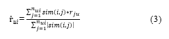
There are several methods for predicting rating, such as weighted average (WA), mean centering (MC), and Z-Score (ZS) [12]. In this study, we use the weighted average method. Correlation value with the top 50 users then used as a weighting factor in order to calculate predicted rating by weighted average as shown in Eq. (3) [12]:

where:

• sim(i,j) is the output of PCC of user i and j similarity
• r_ju is actual rating from user j of item u
• _ui is predicted rating from user u of item i

In CF, we split data into two sections: training and testing. First, we take 5 given ratings by each user and use it as a testing data. Therefore, we have 376,617 as training data and 100,000 as testing data. While predicting test data, the model could output NaN values, so we do not consider when calculating errors.

3.3.2. Neural Collaborative Filtering

Neural collaborative filtering approaches combine general matrix factorization with neural network matrix factorization as shown in Figure 3. This model combines linearity of GMF and non-linearity of neural network in modelling user-item interaction. This model was built by using Keras. Extra preprocessing was implemented when building this model because our input data consist of strings. We then use labelencoder provided by the sklearn library to encode and decode user and music id. Encode is necessary to build the model while decode is used when predicting rating for the user.

For each input, that is: users and music, we create embedding or latent factor with a size of 64 for each item. Then, we multiply item and user embedding as a layer for general matrix factorization (GMF). For the neural network layer, it aims to learn user-item interaction representing predicted rating matrix. Concatenating the item vector with the user vector has been widely used in multimodal deep learning network. However, it does not consider user-item interaction [5]. So, we use a multi layer perceptron (MLP) to learn the interaction function. First, we concatenate item and user embedding and use four hidden layers with 0.25 as a dropout rate. For each hidden layer we implement a linear activation function, ReLu R(x) as shown in Eq. (4). The value of R(x) ranges from 0 to infinite. Then, we concatenate GMF results with the matrix generated from the MLP layer as NeuCF layer. Last, the output of NCF is given by using ReLu activation function on NeuCF layer’s output. The formula used in NCF model are shown in Eq. (5) – Eq. (7) [5].

Figure 3: Structure of Neural Collaborative Filtering

For all formulas above, p_u and q_i denotes user and item embedding respectively. We define this task as a linear regression problem as we intend the output of NCF is the predicted rating value. Therefore, we use mean square error (MSE) as the loss function. Parameters used in this model are shown in Table 1.

 Table 1: NCF Model Parameters

Variable	Value
Batch size	64
Epoch	10
Learning rate	0.001
Optimizer	ADAM

In the neural collaborative filtering approach, we split the data into training, validation, and testing data. The percentage of testing data is 20% of all data and 80% for training. The training data is then split into training and validation, with a percentage of the total data validation of 20% of the training data. Therefore, we have 301,285 as training data, 75,322 as validation data, and 94,152 as testing data.

3.4. Evaluation

Since the recommendation system output is predicted rating, we use regression evaluation metrics. We use mean absolute error (MAE), Mean Absolute Percentage Error (MAPE), mean square error (MSE), and root mean square error (RMSE) for the calculation. The evaluation and comparison of our music recommendation system presented as a value of actual and predicted music rating. The formula of each evaluation metrics is shown in Eq. (8) – Eq. (11):

Where x and y represent predicted and actual value respectively.

4. Experiments

Our experiments take two steps, which are searching the best architecture used for NCF and comparing it with user-based CF. Table 2 and Figure 4 below shows the performance of NCF given different architecture on validation data. We test the model using 32, 64, and 128 latent vector factors or dimensions with 3 and 4 hidden layers. We use 3 and 4 hidden layers based on experiments by [5] which shows that 4 hidden layers results in better NDCG@10 value and 3 hidden layers once give the best NDCG@10 value. For every number of latent vector dimension, it is true that 4 hidden layers model gives less error than with 3 hidden layers. It also showed that 64 latent factor dimensions gives better error performance with about 5 value difference between the lowest error of 32 and 64 latent factors.

Table 2: Neural Collaborative Filtering Performance with Different Architecture

Layers	Factor	Highest Error	Lowest Error	Average Time to Build
3	32	29.123	20.271	13 minutes
	64	26.097	16.480	29 minutes
	128	25.655	24.086	55 minutes
4	32	25.799	15.879	15 minutes
	64	25.201	15.697	30 minutes
	128	25.397	23.676	57 minutes

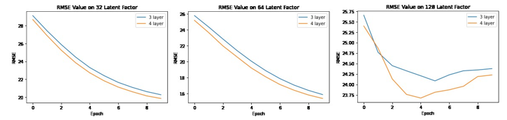Figure 4: RMSE of Neural Collaborative Filtering on Testing Data

Evaluation metrics of CF and NCF shown in Table 3 below are calculated based on the 94,152-test data. Based on the result, it is shown that NCF is better than user-based CF, as it has lower error calculated with MAE, MAPE, MSE, and RMSE. Other than that, CF error has a big difference with NCF with about two times larger. These errors seem to be larger than other research mentioned before because we use a wider range of 0-100 for each rating. It is not surprising since there are some limitations in PCC. Some of the important limitations by PCC are that similar users could only be calculated if there is an overlap over the rated items and due to CF sparse data makes PCC results NaN measure [15].

Table 3: Collaborative Filtering and Neural Collaborative Filtering Performance

Method	MAE	MAPE	MSE	RMSE
CF	14.866	66.118	645.786	26.107
NCF	7.933	28.591	246.422	15.697

Table 4 below shows the predicted rating by using CF and NCF. We use 3 users given 7 sample music to see the difference between actual and predicted rating by both CF and NCF. The closest difference means that the framework predicts better results. NCF framework gets a 21/27 score and reflects that NCF provides more appropriate and optimal recommendations compared to CF.

Table 3: Sample of Recommendation Score

# User	# Song	Actual	CF Score	NCF Score	Winner
1	1	34	43.666	25.124	NCF
	2	13	28.5	10.368	NCF
	3	20	54.75	40.449	NCF
	4	17	13.3	18.745	CF
	5	17	19.66	22.226	CF
	6	3	27	25.456	NCF
	7	6	26.8	25.338	NCF
2	1	5	20.4	17.052	NCF
	2	50	58	51.9	NCF
	3	20	54.75	40.449	NCF
	4	5	13.5	13.961	CF
	5	5	17.666	6.296	NCF
	6	5	23.375	6.747	NCF
	7	11	85	34.424	NCF
3	1	33	30.2	26.475	CF
	2	33	23.25	29.868	NCF
	3	66	44	26.472	CF
	4	33	16.666	30.487	NCF
	5	33	37.5	39.8	CF
	6	33	13.666	40.82	NCF
	7	66	33.2	44.707	NCF

Table 3 and 4 represent NCF framework is better than CF alone as it gets less error in predicting rating. Unfortunately, NCF needs more time to build a model with approximately 25-30 minutes with our model using Google Colaboratory GPU runtime. However, it is worth implementing NCF as it predicts more accurately and faster than user-based CF when using pre-build NCF model. The NCF model needs 5.24 seconds while CF needs 12.16 seconds in recommending music. Therefore, the NCF model must be trained first and stored so that in its application, it is only necessary to load the model.

The experimental results were obtained by following the stages, methods, and architecture described in Chapter 3. The parameters described in Chapter 3 are the best parameters to get optimum results based on several experiments such as changing the number of latent factor dimensions and the number of hidden layers. Other than that, we also consider the time to build the model with the difference of the errors.

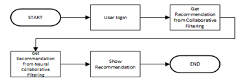Figure 5: Application Workflow

The disadvantage of doing a load model is that it cannot cope with significantly changing conditions. The model is trained with existing data, if there is a change in behaviors, the model cannot handle it. To overcome this, the model must be trained regularly so that changes in user habits can be learned and the system provides appropriate recommendations. In this application, model training is carried out periodically using recurring jobs. With the recurring jobs that carry out training with the latest data, it is hoped that it can overcome significant changes in user behaviours.

An example of a user interface of our application can be seen in Figure 6. After the user logs in, 2 recommendation options will be given, using CF and NCF, this process on our application shown in Figure 5. On that page, the predicted rating for each recommended music is also displayed. There is no identical music on the top 9 recommendations based on CF and NCF. In NCF the predicted ratings are more varied rather than CF results.

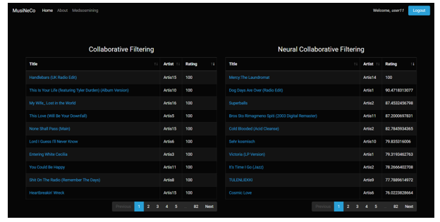Figure 6: Music Recommendation Application

5. Conclusion

Our study focuses on NCF then compared with CF approach on music dataset. From the results discussed in Chapter 4, it can be concluded that NCF produces better recommendations than CF in terms of errors, predicting ratings, and time used to predict. It is unsurprising that NCF gives better performance since it learns the user and music embeddings that more similar users in the context of preferred music are closer to each other in the embedding space rather than single correlation calculation performed on CF. Moreover, recommendation model from NCF could be used repeatedly on giving recommendation without recalculating similarity between users when needed. However, building NCF model needs more powerful computation power due to massive matrix manipulation needed.

In addition to making comparisons between CF and NCF, we also make comparisons with several model parameters to the NCF model in order to obtain an optimal model. Model with more hidden layer may converge in a higher level of abstraction. It is proved in this study that four hidden layers model gives smaller error paired with small time difference when building the model compared with three hidden layers model. The result of this study can be implied to increase people’s engagement with digital online music applications as it provides sufficient recommendations according to the user preference.

Although neural collaborative filtering has better results than collaborative filtering, this method has a weakness in terms of preparation time because it has to go through the build and training model stages. This stage takes a long time, so the alternative is to save the trained model and load the model to get recommendations. To solve the process time problem, the implementation of the application does not do real-time training instead, it loads a trained model. Further research on recommendation systems could contribute in proposing a new approach or combining several approaches to improve system performance, either in terms of times, effectiveness, errors, accuracy, or other performance metrics.

Conflict of Interest

The authors declare no conflict of interest.

Acknowledgment

This work is supported by the Directorate General of Strengthening for Research and Development, Ministry of Research, Technology, and Higher Education, Republic of Indonesia, as a part of  Penelitian Terapan Unggulan Perguruan Tinggi Research Grant to Binus University titled “Pengembangan Sistem Rekomendasi Lagu Menggunakan Neural Collaborative Filtering” or “Song Recommendation System Development Using Neural Collaborative Filtering” with contract number: 25/E1/KPT/2020, 225/SP2H/LT/DRPM/2019, 088/LL3/PG/2020, 039/VR.RTT/IV/2019.

1. T. Schäfer, “The goals and effects of music listening and their relationship to the strength of music preference,” PLoS ONE, 11(3), 1–15, 2016, doi:10.1371/journal.pone.0151634.
2. D. Sánchez-Moreno, A.B. Gil González, M.D. Muñoz Vicente, V.F. López Batista, M.N. Moreno García, “A collaborative filtering method for music recommendation using playing coefficients for artists and users,” Expert Systems with Applications, 66, 1339–1351, 2016, doi:10.1016/j.eswa.2016.09.019.
3. D. Jayashree, S. Goutham Manian, C. Pranav Srivatsav, “Music recommendation system,” Asian Journal of Information Technology, 15(21), 4250–4254, 2016, doi:10.3923/ajit.2016.4250.4254.
4. H. Liu, Z. Hu, A. Mian, H. Tian, X. Zhu, “A new user similarity model to improve the accuracy of collaborative filtering,” Knowledge-Based Systems, 56, 156–166, 2014, doi:10.1016/j.knosys.2013.11.006.
5. X. He, L. Liao, H. Zhang, L. Nie, X. Hu, T.S. Chua, “Neural collaborative filtering,” 26th International World Wide Web Conference, WWW 2017, 173–182, 2017, doi:10.1145/3038912.3052569.
6. Y. Hu, C. Volinsky, Y. Koren, “Collaborative filtering for implicit feedback datasets,” Proceedings – IEEE International Conference on Data Mining, ICDM, 263–272, 2008, doi:10.1109/ICDM.2008.22.
7. N. Sivaramakrishnan, V. Subramaniyaswamy, S. Arunkumar, A. Renugadevi, K.K. Ashikamai, “Neighborhood-based approach of collaborative filtering techniques for book recommendation system,” International Journal of Pure and Applied Mathematics, 119(12), 13241–13250, 2018.
8. A. Gunawardana, G. Shani, “A survey of accuracy evaluation metrics of recommendation tasks,” Journal of Machine Learning Research, 10, 2935–2962, 2009.
9. A.S. Girsang, A. Wibowo, Edwin, Song Recommendation System Using Collaborative Filtering Methods, 2019, doi:10.1145/3369199.3369233.
10. A.K. Azmi, N. Abdullah, N.A. Emran, “A hybrid knowledge-based and collaborative filtering recommender system model for recommending interventions to improve elderly wellbeing,” International Journal of Advanced Trends in Computer Science and Engineering, 9(4), 4683–4689, 2020, doi:10.30534/ijatcse/2020/71942020.
11. S. Ayyaz, U. Qamar, “Improving collaborative filtering by selecting an effective user neighborhood for recommender systems,” Proceedings of the IEEE International Conference on Industrial Technology, 1(2), 1244–1249, 2017, doi:10.1109/ICIT.2017.7915541.
12. P.K. Singh, M. Sinha, S. Das, P. Choudhury, “Enhancing recommendation accuracy of item-based collaborative filtering using Bhattacharyya coefficient and most similar item,” Applied Intelligence, 50(12), 4708–4731, 2020, doi:10.1007/s10489-020-01775-4.
13. Y. Zhang, D. Liu, G. Yang, L. Hu, “Quantization-based hashing with optimal bits for efficient recommendation,” Multimedia Tools and Applications, 79(45–46), 33907–33924, 2020, doi:10.1007/s11042-020-08705-z.
14. X. Chen, D. Liu, Z. Xiong, Z.-J. Zha, “Learning and Fusing Multiple User Interest Representations for Micro-Video and Movie Recommendations,” IEEE Transactions on Multimedia, 9210(c), 1–1, 2020, doi:10.1109/tmm.2020.2978618.
15. L. Sheugh, S.H. Alizadeh, “A note on pearson correlation coefficient as a metric of similarity in recommender system,” 2015 AI and Robotics, IRANOPEN 2015 – 5th Conference on Artificial Intelligence and Robotics, 2015, doi:10.1109/RIOS.2015.7270736.

(Click Here)