1.Introduction

With the development of new applications in numerous areas, wireless sensor networks (WSNs) have gained a vast reaction from academia and industry. Applications for the future include monitoring of vegetation and the environment, search and rescue processes, object tracking in hospitals, monitoring of patients, and military applications. Because of technological development, small, cheaper sensor nodes have been developed that consume less power and feature capabilities like sensing, data storage, computer technology, and wireless communication.

Localization among others, architecture, deployment, synchronization, calibration, quality of service, and security are the key and difficult part of many WSN applications. The sensor data has to be attached to measured data in order to make this important for location since it is essential to monitor and record broad information like acoustic, visual, thermal, and seismic or any other type of measured observation. For example, the place or part of the farm from which the data is collected would be required for the person monitoring a big vegetation farm, with a wide variety of vegetables, since various vegetables have different special needs. Reporting   Object origin, node location is required so as to support or answer group querying, routing and network coverage questions. Research into the problem of node location has provided a number of solutions over the course of the decade. Overall, most of the time there is a compromise between localization accuracy, computer complexity, and technology energy efficiency according to their application needs.

A large number of space-dispersed sensor nodes is usually used in a WSN such that the location of the sensor node when the nodes are used is unable and inefficient. Sensor nodes may also be relocated from their original position. An algorithm is therefore necessary for an independent assessment of the location of the node. In this research paper, a new location scheme for neural network-based nodes is proposed. In order to address the node location problem, the Received Signal Strength Indicator (RSSI), is utilized to evaluate the coordinates and location of WSN nodes. Contributions are as follows:

Is RSSI an appropriate component for WSN node location? We use RSSI to determine where the sensor nodes are located and explain how RSSI is suitable for locations. There will not be a need for additional hardware because sensor nodes are openly outfitted with RF modules for wireless communication. Multi track fading and noise, however, can contaminate the RF signal and thus affect the RSSI value through a noise-to-signal correction.

Also, of the utmost importance is the choice of the evaluation model. A 2D indoor environment that is determined by the x and y co-ordinates is considered in this research. A single node of anchor requires directional steering antennas, which directly boosts the sensors’ cost and electricity consumption. Therefore, the two or more anchor nodes with different configurations explain the best configuration used for the anchor nodes.

A new 2D indoor locating system based on a neural network is introduced. For an accurate localization, the global positioning system can be used. The use of GPS does require the attachment of external hardware to the sensor nodes, thereby increasing cost and electricity consumption. In addition, a GPS viewing line is required and is therefore not applicable to indoor environments.

A neural feed network is used for the proposed indoor position process. A variety of neural network configuration sets have been tested, and Bayesian regularisation (BR), Levenberg-Marquardt (LM), resilient back propagation (RP), Scaled Conjugate Gradient (SCG) and Degree Descent (SCG) are the best neural network training and implementation (GD).

2.Literature survey

In [1], the authors presented a survey on machine learning algorithms for WSNs. They have presented techniques to identify intrusion by merging clustering and deep neural network methods and discussed machine learning-based localization techniques for WSN such as fuzzy logic, k-means + fuzzy-c-means, CNN+SVM, ANN, SVM. Also discussed ML-based congestion control strategies. Logic-based cram detection and control systems have been configured for efficient and active queue management as the basis for minimizing packet loss. It can be carried out in three stages. Second, it senses congestion in the second it modifies congestion control and by balancing the flow it recovers from the congestion.

In [2], the authors have suggested a new distance measuring capability using the Adaptive Neural Fuzzy Inference Scheme to render model, map RSSI to the precise T-R distance and experiments prove feasible.

In [3], the authors has proposed an adaptable model dependent on the neural organization and lattice sensor preparing stage for exact limitation of sensors. Recreation results show that the area exactness can be expanded by expanding the framework sensor thickness and the number of passages. The author proposed and explored a confinement procedure for WSNs utilizing NN. They think about NN for building adaptable planning among RSS and the situation of the sensor hubs. In this method, the NN is prepared to utilize the RSS estimations of the lattice sensors. The positive highlights of the framework are its dependence against the adjustment in the RSS estimations with time and no requirement for the additional course of action of equipment. The organization’s preparation is refreshed with a standard timespan to limit area mistake. Simulation experiments demonstrate that the area exactness can be expanded by expanding the matrix sensors’ density and APs.

Nowadays for enhancing the accuracy of localization in the Range-Free approach is more focused. In [4], the authors introduced many algorithms to improve accuracy such as BP artificial neural network (BP ANN). Rather than the amorphous algorithm is very easy to develop, and it will generate huge errors in the localization procedure. For resolving the issue and to diminish localization error, presented an improved localization algorithm. A widely utilized model in neural networks (NN) is BP NN. BP algorithm is a NN of three-level. The methodology used for the detection of network weight and the threshold between BP algorithms with minimal error and recursive technology is known as the deepest descent. BP ANN practitioners are incredibly self-organizing and self-learning, error replication, and a minimal theory of error in error optimization.

In [5], authors presented a study on localization in WSN by utilizing neural networks (NN). This study analyses localization algorithms and their advantages and disadvantages. They Discussed localization, localization classification methods, localization classification algorithms, and the pros and cons.

In [6], authors submitted comparable analyses of the localization WSN localization networks of Sigmoidal Feed ANN (SFFANNs) and Radial Base Function (RBF). The system proposed uses the Obtained Signal Force Indicator (RSSI), a static node calculated on a grid of 100 x 100 m2 of the three anchor nodes. The key aim of the SFFANNs’ and RBF network system comparative analysis is the development of an efficient WSN localization structure. Both ANN models approximate the position error by using RSSI values. Quality comparison has been done with respect to standard deviations, mean position errors, and statistical parameters of R-square. MLP has the best efficiency, shown by simulation outcomes, where accuracy is considered.

In [7], the RBF network has been reviewed by the authors for the implementation of the WSN position method. For reasons of faster convergence and the lowest measurement rate, the RBF-based localization architecture should be evaluated. The analyses of RBF in this paper have been a probabilistic NN and general regression NN. For designing an efficient localization method, the suggested technique may be used. To minimize position errors, the predictive location algorithm proposed by  the authors [8] relies on RBF NN. An algorithm detains moving node standards inherent in it and learns them from them. A field of mobile nodes can be expected by removed traveling highlights. Reproduction findings confirm that these calculations will be more reliable in the visually impaired interval to understand detailed localizations.

In [9], the authors proposed computationally – cheap arrangements rely upon support vector machine (SVM) and twin SVM learning algorithms where network nodes right off wanted signal. At that point, the network is trained to determine nodes in the region of source; subsequently, locale of the function is distinguished. At last, centroid of event region is assessment of source area. Re-enactments show the productivity of the proposed techniques. SVMs are integral tools for regression and classification which depend on the statistical learning hypothesis. Contrasted and other ML strategies, for example, ANNS, SVMs have a superior speculation ensure. SVM separates the data tests of 2 classes by deciding a particular hyperplane in input space. This hyperplane boosts the partition among 2 classes by taking care of a quadratic programming issue whose arrangement is around the globally optimal.

In [10], the author has examine the reasonableness of a portion of these algorithms while investigating diverse compromises. In particular, authors initially figure new method of characterizing many feature vectors for planning localizing issues onto diverse AI models. Instead of regarding localization as a classification issue, as accomplished in the majority of detailed work, authors treat it as a regression problem. Authors have contemplated an effect of varying network parameters, for example, anchor population, network size, transmitted signal power, and remote channel quality, on confining precision of the models. Authors have additionally considered the effect of sending anchor nodes in  the framework as opposed to putting the nodes arbitrarily in deployment areas. Their outcomes have uncovered fascinating experiences while utilizing the multivariate regression model and SVM regression model with an RBF. Various models have been characterized for various ML algorithms. A portion of the normally utilized models incorporates neural networks, multiple linear regression model, linear regression model, SVM with various kinds of kernels, Logistic regressions or classifications, k-nearest neighbours (KNN), and random forest (RF) clustering.

In order to address the Wireless Sensor Networks (WSN) localization accuracy problem in [11], the authors have suggested the latest Methodology for Localization Backpropagation Network (BPNN). At first, node localization calculations are provided with range intervals and signal power, and on BPNN the parameters solve easily. In a simulation experiment, the main factors of NS2 and MATLAB are also evaluated. The results show that this technique is successful in comparison with other localization algorithms and can minimize localization errors effectively.

In [12], the authors proposed ANNs way to deal with localization in WSN through change of ANNs structures utilizing Genetic Algorithms. Populace of feed forward ANNs composing their structure in genetic code is developed more than 20 ages. Every individual is assessed through the preparation of training of ANN and further estimation of its root mean square error for all testing set. The RSSI estimations were utilized as ANN inputs to localize hubs. The methodology is to collect information from the ANNs under an input reactivated static 26 x 26 meter indoor organizational climate, which consists of eight anchor hubs, under a reactivation of the static 26×26 meter indoor organization environment. The methodology has been used. Hereditary calculations of MATLAB and fake neural organizations were used for stashing tools.

In [13], the authors emphasise the comparison and study of MLPNN and RBFNN for the creation of a position system in WSNs. Various sensor node collection were evaluated using both MLPNN and RBFNN along with the mean square error of various input data sets. Their simulation findings effectively suggest that MLPNN is more reliable with respect to localization than RBFNN.Use the “Insert Citation” button to add citations to this document.

In [14], the authors suggest a new algorithm for localizing the sensor nodes using virtual anchor nodes. VAN is located in its system with minimum anchor nodes. The goal of their work is to improve the accuracy of the position by optimizing the location ratio and minimizing the costs of several anchor nodes.

In [15], the author explained the localization based on ANN in WSN. Localization refers to the issue of finding the location or position of sensor nodes in a network. But localization problem is still an open challenge in WSN. Author analyzed and classified existing works on localization algorithms that uses ANN. ANN algorithms were identified based on how they were utilized in the localization processes; noise characterization, model construction, training phase optimization, clustering, and prediction. Author also discussed about the features and related work about it and how to improve the accuracy of previous localization using ANN.

In [16], the authors proposed an approach known as ANN approach for moderating the reaction of mixed noise sources and harsh factory conditions on the localization of the wireless sensors. They have focused on investigating the effect of blockage and ambient conditions on the accuracy of mobile node localization. They have added a simulator for simulating the noisy and dynamic shop conditions of manufacturing environments, also for analyzing the proposed neural network.

In particular, in networks with sparse anchor deployment, cooperative localization improves the accuracy of position estimates. In [17], the authors presented implementation of it in low-cost WSN that are low-power. A WSN hardware platform with ultra-wideband range and communication is shown and the implementation of a cooperative localization algorithm based on belief propagation is addressed. The key sources of error are addressed and indoor tests of the device are performed using a simple channel access scheme and a standard ranging process.

In [18], the authors presented an enhanced centroid localization algorithm for WSN. One of the main technologies in the WSN is node localization. The center position algorithm depends entirely on the size and distribution density of the anchor nodes, but they are distributed randomly and their density is small. Given the conventional centroid localization algorithm, an enhanced centroid localization algorithm is vulnerable to the effect of network deployment status and the current situation of low positioning accuracy. Second, the idea of reference anchor nodes is implemented by bringing weight thought into the measurement method of node coordinates.

This template, modified in MS Word 2007 provides authors with most of the formatting specifications needed for preparing electronic versions of their papers. All standard paper components have been specified for three reasons: (1) ease of use when formatting individual papers, (2) automatic compliance to electronic requirements that facilitate the concurrent or later production of electronic products, and (3) conformity of style throughout the conference proceedings. Margins, column widths, line spacing, and type styles are built-in; examples of the type styles are provided throughout this document and are identified in italic type, within parentheses, following the example. Some components, such as multi-leveled equations, graphics, and tables are not prescribed, although the various table text styles are provided. The formatter will need to create these components, incorporating the applicable criteria that follow.

3. Methodology

An ANN, also known as the network of neurons, offers a simple way of revealing valued and true functions as examples. ANN uses a supervised curriculum. Inputs and outputs to the ANN are given to learn and create a correct model. The classification and regression dilemma is normally tackled. Typically, the artificial neuron network has 3 layers, input layer, hidden layer(s), and finally output layers.

Neural feedback and feedback networks form two classes of neural networks. In a neural feed network, the outcome is fed from one layer of neurons to the next layer, no layers are skipped during this process, and the system has no feedback. The position is composed of three major neural networks: MLP, the Recurrent Neural Network and, the RBF.

It is to be noted that RSSI values are very unpredictable and vary under ambient noise and sensor mobility. The benefit of a neural network is that prior environmental and noise propagation is not needed. More precision is achieved through a neural network compared to other approaches such as Kalman filters. Comparing other neural network types, for the study the compromise between MLP neural accuracy and the network memory requirement was chosen.

Figure 1: A general feed-forward neural network structure with four inputs and three outputs.

3.1. Network Model

WSN model for region assessment of static sensor nodes. Static nodes are moved to region of recognition and the node of mobile

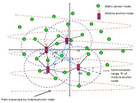Figure 2: Illustration of broadcasting and reception of beacon signal from a Mobile Anchor and static sensor node respectively.

anchor (MA) ready for intersection. In addition, in the fig, the way MA navigates. 2.

It is assumed that R is a contact range of the MA hub. MA has a GPS recipient and knows its location often. The MA is sending beacon signal at a fixed “Live” interval with an id, transmission radius, current location, transmission power and format shown in figure 2. Before the MA node moves around the sensor area, the administrator determines the ‘alternative’ intervals.

MA_id

MA current Position (x, y)

Transmitted power

Transmission range ‘R’

Figure 3: Packet format of beacon message

Any static sensor node in MA node’s “R” range receives a signal from the beacon. A table called Mobil Anchor Location (MAP), as represented in Table 1, is retained in every static sensor Node.

When static sensor node beacon signals are obtained, X-y coordinate values are extracted from signal and stored in the MAP table in corresponding fields. The distance is determined according to the signal power obtained and stored in the Chart Table.

Consider scenario in Figure 2, let  and  be the MA positions throughout its traversal time and having   ,  and  as their coordinates. Static sensor node S1, at position δ whose co-ordinate is , receives beacon signals when MA is at position  and  and stores their x-y co-ordinate values into MAP table. Similarly, S1 receives beacon signals when it comes into MA node proximity.  Eventually, x-y co-ordinate values are extracted from received signal and stored into MAP table.

3.2. RSS Measurement

Distance from the MA node at position I to the static node S1 at position (x0, y0) is referred to as a correspondence to r (i), as seen in the following equations; (R2) The noise free RSS or received power at S1, denoted by

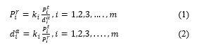If the beacon signals received by the static node i=1, 2… m number, the transmitted power is , the power received is , and the propagation constant is α, k (i)denotes other environmental variables that influence the received power.

Range related measurement can be modeled, as expressed in (R1)

Every static node calculates  for each received beacon signal and stores into MAP table as demonstrated in table 1.

Table 1: MA Positions stored at static sensor node

X-co-ordinate	Y-co-ordinate	Distance (r)
(x1)	(y1)	r1
(x2)	(y2)	r2
(x3)	(y3)	r3
(x4)	(y4)	r4
·	·	·
·	·	·
( xm)	(ym)	rm

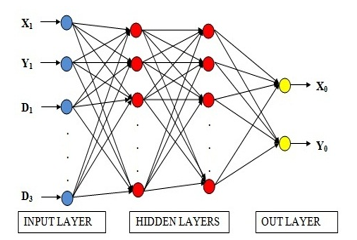Figure 4: Multi-layer perceptron neural network

3.3. Multi-Layer Perceptron Neural Network Model

Neural network model (framework), initially trained with training dataset. Proposed system consisting of Multilayer Perceptron neural network [MLPNN] model having input layer, one or more hidden layers and output layer.

Nine inputs are passing to MLPNN, consisting of three different positions of MA with respect to distance from sensor node. Hidden layer having various neurons. Each neuron, having transfer function to find out weights of each connection between inputs to hidden layer neurons. Output layer having two neurons produces the location coordinates of unknown sensor node. Activation function (linear or nonlinear) is used to calculate location of sensor nodes.

3.4. Algorithm

The multilayer perceptron algorithm is as follows:

Step 1: Initialization: Arbitrary values are used to trigger all networks and thresholds, which are consistently distributed across a limited range. If these values are 0, gradients will also be computed to 0, if and only if there will be no direct relation between input and output and network. More training trials, with various initial weights, are planned to have the best cost-effectiveness. If the initial values are sufficiently high, however these units appear to be saturated.

Step 2: A new period of formation: an era means all the examples are presented in the training set. Training on the network typically requires further training times. The weights are calibrated for statistical rigour, only after the test vectors are applied on the network. Therefore, after each model in the training set and after the end of the training stage, weights must be memorised and adjusted, the weights changed only once. There is a “online version, simpler, which directly updates weights, in which case there may be the order in which the network vectors are displayed. Both weight gradients and current error have been initialised at 0 (alternative to 0) and E=0).

Step 3: The forward propagation of the signal

An example from the training set is applied to the inputs. Outcomes of neurons from hidden layer are computed:

Where n is hidden layer number of inputs for neuron j and f is sigmoid activation.

Real network outputs are measured:

Where m is the input number from the output layer of neuron k.

Error updated by epoch:

Step 4: Backward error propagation and weight correction. Neuron error gradients are computed in the output layer:

where f’ is the activation derivative function. A mistake occurs as

If we use the single-pole sigmoid (equation 1, its derived is:

Furthermore, the single-pole sigmoid is the function used. Then it becomes equation (10):

The weight gradients from the secret layer to the output layer are updated:

The gradients of the neuron errors are determined in the secret layer:

where l is the number of network outputs.

The weight gradients of the input layer are modified with the hidden stage.

Step 5: A new version. A new one. If the current training cycle still has test vectors, pass stage 3. If not the weights of all the links are changed according to the weight gradients:

Where μ is the rate of analysis. When a stage is over, we check if it meets the termination condition (E < E_max or a maximum number of periods of training have been achieved). Otherwise, we will move on to phase 2. If so, the MLP algorithm is over.

3.5. Simulations

On a PC with an i5 processor with an 8 GB RAM processing speed of 3.50 GHz, simulations can be brought. Sensor nodes are positioned on the grid intersection points and are first learned to locate as seen in the Figure. 5.

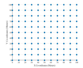Figure 5: Illustrate the deployment of Sensor nodes and Mobile anchor node

The trained network with numerous training algorithms has placed localised sensor nodes on arbitrary points on the grid. The research is conducted. The node position is determined with the positioning information of the moving anchor node. The network is taught and checked using a handheld anchor node with the initial position to determine network efficacy (0.5, 0.5).

The sensor nodes are initially installed in a fixed location on the grid during testing. The handheld anchor node that has a set network gap has been deployed. Each mobile anchor node interval ‘t’ sends its present position (X and Y coordinates) to sensor nodes that fall within its radio frequency spectrum. Each sensor node shall compute its current position using the proposed position algorithm by obtaining a minimum of three separate location information from mobile anchor node positions.

To determine the position of sensor nodes in the same grid, a further test of the qualified network is carried out. The nodes of the sensor were spread around the test grid uniformly. The testing is seen via the coordinate grid.

4. Results and discussion

For this study 5 different training algorithms BR, LM, RP, GD and SCG have been used for formation of the neural network, requiring supervised learning.

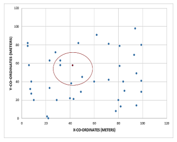Figure 6: Illustration of Mobile anchor node with random deployment of sensor nodes

A neural network. Several testing functions with a different number of layers and nodes have been conducted. There are optimal results from network of 3 layers with a 9-12-2 structure. There were 9 neurons in input layer, hidden layer with 12 neurons and two in the output layers. Hyperbolic sigmoid tangent activation function for hidden layers, whereas pure line function in output layer has been used. This structure was utilized for the evaluation of the performance of the following anchor node configurations with different numbers of anchors.

An experiment was performed. 5 different BR, LM, RP, GD and SCG training algorithms for the formation of a neural network that require supervised learning have been used to this study. A network of neural components. A number of test functions have been performed with different layers and nodes. A network of three layers with a structure 9-12-2 produces optimal results.

where n is the overall number of test sets and exact position ( , ) and estimated position of sensor node in i^th test dataset is ( , ).

The above mobile anchor node configurations were used for assessments of the performance of various anchor numbers. The average location error during this phase is illustrated in Figure 7. Figure 8 shows the time required for the network to train using different training algorithms.

Figure 7: Illustration of localization error of different training algorithm with mobile anchor.

In Figure 7, Depicts different training algorithms have compares with localization error. The BR training algorithm is having less average error as compared to other training algorithms.

Figure 8: Illustrate time taken to train neural network for different training algorithms with mobile anchor

In Figure 8. Shows the training time taken by the ANNN model for different training algorithms. LM, RP and SCG are taking less training time and BR and GC training algorithms are taking more training time.

Cost of the network will be reduced with using one mobile anchor agent. Estimated Mean Localization Error (Meters) for different number of sensor nodes using BR training algorithm is shown in Figure 9 for the communication range of mobile anchor node that is R=40 meters, 60 meters and 80 meters.

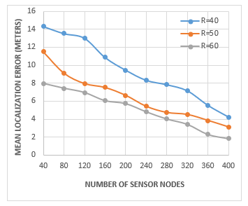Figure 9: Estimation error when varying communication range.

In Figure 10. Depicts convergence accuracy of mobile anchor node with different time stamps for broadcasting their location information to static sensor nodes using BR training algorithm.

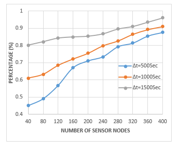Figure 10: Convergence accuracy for various regular intervals.

5. Conclusions

The use of ANN has been suggested for an effective 2D localization algorithm for WSN. The RSSI signal values from the mobile anchor node are the entry to the proposed process. Since every mobile anchor node is fitted with wireless RF modules, no external hardware is necessary. The approach proposed is therefore , energy-efficient and uses just a two-way message to obtain the location inputs. As in the proposed system, only one mobile anchor node is used, even the cost is minimized. It is however, advisable to use the RSSI value of the mobile-based anchor Node beacon request signals, which may further reduce the location error. The following is recommended.

In order to obtain the finest neural network for localization, the BR training algorithm is evaluated to give the best results. Hence, the training time for this algorithm is quite high compared to other methods such as LM, RP, and SCG. It is therefore recommended that the BR method is used when offline training is performed as in this case. The LM method is recommended for applications requiring online training.

Conflict of Interest

The authors declare no conflict of interest related to this paper.

1. D. Praveen Kumar, T. Amgoth, C. S. R. Annavarapu, “Machine learning algorithms for wireless sensor networks: A survey,” Information Fusion, 49, https://doi.org/10.1016/j.inffus.2018.09.013.
2. X. Feng, Z. Gao, M. Yang, S. Xiong, “Fuzzy distance measuring based on RSSI in Wireless Sensor Network,” 2008 3rd International Conference on Intelligent System and Knowledge Engineering, https://doi.org/10.1109/iske.2008.4730962.
3. M. S. Rahman, Y. Park, K. D. Kim, “Localization of Wireless Sensor Network using artificial neural network,” 2009 9th International Symposium on Communications and Information Technology, https://doi.org/10.1109/iscit.2009.5341165.
4. L. Zhao, X. Wen, D. Li, “Amorphous Localization Algorithm Based on BP Artificial Neural Network,” International Journal of Distributed Sensor Networks, 11(7), https://doi.org/10.1155/2015/657241.
5. K. Madhumathi, Dr. T Suresh, “Localization of Mobile Wireless Sensor Node Using Randomized Feature Sample of Estimated RSSI Value,” Journal of Advanced Research in Dynamical and Control Systems, 11(11-SPECIAL ISSUE), https://doi.org/10.5373/jardcs/v11sp11/20192943.
6. A. Payal, C. S. Rai, B. V. R. Reddy, “Comparative Analysis of Sigmoidal Feedforward Artificial Neural Networks and Radial Basis Function Networks Approach for Localization in Wireless Sensor Networks,” International Scholarly and Scientific Research & Innovation, 10(7), https://doi.org/doi.org/10.5281/zenodo.1125123.
7. A. Payal, C. S. Rai, B. V. R. Reddy, “Analysis of Some Feedforward Artificial Neural Network Training Algorithms for Developing Localization Framework in Wireless Sensor Networks,” Wireless Personal Communications, 82(4), https://doi.org/10.1007/s11277-015-2362-x.
8. C. Xiao, & N. Yu,” A predictive localization algorithm based on RBF neural network for wireless sensor networks,” 2015 International Conference on Wireless Communications & Signal Processing (WCSP), https://doi.org/10.1109/wcsp.2015.7341145.
9. S. Javadi, H. Moosaei, D. Ciuonzo, “Learning Wireless Sensor Networks for Source Localization,” Sensors, 19(3), https://doi.org/10.3390/s19030635.
10. G. Bhatti, “Machine Learning Based Localization in Large-Scale Wireless Sensor Networks,” Sensors, 18(12), https://doi.org/10.3390/s18124179.
11. C. Zhou, L. Wang, L. Zhengqiu, “The Study of WSN Node Localization Method Based on Back Propagation Neural Network,” Advances in Intelligent Systems and Computing, https://doi.org/10.1007/978-3-319-67071-3_54.
12. S. H. Chagas, J. B. Martins, L. L. De Oliveira,” An approach to localization scheme of wireless sensor networks based on artificial neural networks and Genetic Algorithms,” 10th IEEE International NEWCAS Conference, https://doi.org/10.1109/newcas.2012.6328975.
13. B.K. Madagouda & R. Sumathi, “Analysis of Localization Using ANN Models in Wireless Sensor Networks,” 2019 IEEE Pune Section International Conference (PuneCon), https://doi.org/10.1109/punecon46936.2019.9105871.
14. B.K. Madagouda, R. Sumathi, A. H. Shanthakumara, “Localization of Sensor Nodes Using Flooding in Wireless Sensor Networks,” Communications in Computer and Information Science, https://doi.org/10.1007/978-3-642-29219-4_72.
15. R. Dela Cruz, “Artificial Neural Network-based Localization in Wireless Sensor Networks”.
16. M. Gholami, N. Cai, R. W. Brennan, “An artificial neural network approach to the problem of wireless sensors network localization,” Robotics and Computer-Integrated Manufacturing, 29(1), https://doi.org/10.1016/j.rcim.2012.07.006.
17. B. Etzlinger, A. Ganhor, J. Karoliny, R. Huttner, A. Springer, “WSN Implementation of Cooperative Localization,” 2020 IEEE MTT-S International Conference on Microwaves for Intelligent Mobility (ICMIM), https://doi.org/10.1109/icmim48759.2020.9299096
18. X. Yang, X. Wang, W. Wang, “An Improved Centroid Localization Algorithm for WSN,” 2018 IEEE 4th Information Technology and Mechatronics Engineering Conference (ITOEC), https://doi.org/10.1109/itoec.2018.8740471.

(Click Here)