1.Introduction

This paper is an extension of work originally presented in 15th International Computer Engineering Conference (ICENCO) [1]. The food demand increased due to the huge growth in population so it is essential to increase the food production and try to avoid any production losses. Agriculture has a major impact on food production so monitoring the plants’ performance is very important. In order to avoid any crop losses, agro systems were designed. Remote sensors were used in these systems to measure light, humidity, soil moisture and temperature. The measured data will indicate whether the plants’ performance is good or not and the data will be collected and sent to the user for further action[2, 3]. IoT is a new technology that is used recently in most of the smart systems. Using IoT technology in agro systems allow the plants to express its needs only when it is needed which will allow the efficient usage of resources. There are some challenges that appears in IoT systems, energy optimization is one of the main challenges that faces IoT. It is a major challenge due to the high number of devices that exist in the network which need high energy to keep it active for long time. It is essential to study this challenge as wireless sensors are commonly used in precision agriculture in remote areas and the agro systems depend mainly on sensors’ power so battery drainage will cause the system to stop which isn’t desired [4, 5].

The life time of sensor nodes needs to be long in order for the network to be active and to avoid battery drainage. In this paper, an energy management technique based on intelligent load scheduling is introduced for agro-applications. The battery state of charging and the solar power are the main parameters used in the proposed algorithm to activate or deactivate the loads. Based on the loads’ priority and the availability of power provided by the battery or solar, loads are activated for specific time. The loads’ priority is standard defined as the applications that need to be operating due to criticality are defined based on the standards of agro.

2. Literature Review

Researchers have implemented and introduced some systems using various methods and sensors to monitor the status of plants’ health. It improved the agricultural production and helped in preventing crop losses. In [6], the author illustrated the demonstration of a smart plant monitoring system. The system was enabled to discover any changes occurred in the measurements of light, moisture level and temperature. The plant received its required irrigation and illumination using a machine based curation. An Android device was used by the user in order to enable the user to override an operation which is a machine curated and in this case it is shifted to user based curation instead of machine based curation. In [7], the author explained a system that uses IoT technology in order to control and monitor an agricultural production. The sensors’ data was gathered in the monitoring system from IoT devices and then stored at the database of the cloud in order to be accessible by the users. The users could control the actuators in the controlling system over the internet with the usage of IoT devices.

The main source of power for the systems presented previously is the sensors’ batteries so systems that uses energy efficiently are studied. Energy plays a significant role in monitoring the environment of agriculture. Researchers presented various algorithms which assure the efficient usage of energy using energy harvesting, load scheduling and power reduction techniques. In [8], the author presented a method used in wireless sensor network for managing power efficiently. The system model consisted of three parts: sensing unit, transmitter unit , and power unit. Energy harvesting was used in the power unit as the power source used for charging the battery is the solar energy. Sending and collecting the data was the responsibility of the other two units. The microcontroller is utilized to monitor the sensed signal and if any disorder detected, it would be transmitted to the receiver.

In [9], the author concentrated on elongating the sensor nodes’ life time by minimizing the consumption of energy. A solar cell was utilized to power the system to assure energy sustainability. The minimization of power consumption was achieved by proposing two methods of power reduction. Sleep/wake based on duty cycling was utilized and the second method was integrating the redundant data of the soil moisture with sleep/wake scheme. This research introduced the Sleep/wake on redundant data (SWORD).

In [10], the author presented an algorithm based on devices scheduling in order to optimize and reduce the electricity cost.  Two methods were tested for load scheduling optimization either without the usage of renewable energy or with the usage of it. The results of the implementation showed that the cost is reduced up to 53% when combining the proposed algorithm with renewable energy and in case no renewable energy is combined with the algorithm, the cost is reduced up to 40%.

In [11], the author illustrated an algorithm that depends on electricity cost changes and renewable sources real time output in order to schedule the loads. The scheduling and management of energy was established according to the exchange of sensor data and control demands. It would update the real time output of the renewable sources and determine the devices’ priority. After the sensed data was received, the energy management unit in the system updated the devices’ priority status and the output of renewable sources. The energy management unit would transfer the devices to on or off status if required depending on the energy management and devices scheduling.

In [12], the author discussed various ways to utilize renewable energy in order to assure the efficient usage of energy, ,cost reduction, and handling loads. The scheduling of loads in the used algorithm was depending on time and overload management using multilevel priority. Based on the need of load scheduling during peak demand hour, a duration of time was determined. The loads with medium and high priorities would be activated during this time and the load with low priority would be deactivated. All load would be deactivated in case the limit was exceeded.

3. Proposed Architecture for Energy Efficient Agro Systems

As shown in Figure 1, the proposed architecture consists of four sensors: light sensor, color sensor, soil moisture sensor and temperature/humidity sensor. The proposed architecture is used for monitoring plants’ performance in agro systems. The data measured by the soil moisture sensor and temperature/humidity sensor will be sent to Central Processing Server (CPS) to decide the proper time for irrigation after comparing it with the threshold values. Regarding the other two sensors, the user will take the action required based on the received data that were measured by these sensors in case there were any up normal values detected at the CPS. The goal is to ensure the continuous operation of this system by using energy efficiently to increase the life time of the system. Figure 2 shows a proposed architecture for sensor area network (SAN1) using energy efficient technique.  It depends mainly on two parts:

3.1. Solar panel or battery used as a power source

• The source of power during day is the solar panel. It is used for supplying the loads during day as it is working and the power needed by the loads is available. Some loads will be switched off in case that the solar power isn’t enough for suppling all loads and the rest will be on depending on the available solar power.
• The source of power during night is the battery. The active loads will be supplied by the battery and some loads will be off during night as these loads will not highly affect the system’s operation.

3.2. The loads (sensors and actuators) which are divided into categories according to priority.

• Load 1 (High priority): the high priority loads highly affect the system’s operation. This load must be on most of the time so the deactivation will be during night only in case that the state of charging of the battery is less than the threshold value.
• Load 2 (Medium priority): if the power is enough for supplying medium and high priority loads, this load will be active. It will be deactivated when the power isn’t enough to supply all loads and this will occur mostly during night.
• Load 3 (Low priority): it doesn’t have a huge impact on the system’s operation so it can be deactivated during night. The user can activate this load upon his request if needed during night after checking the battery state of charging if it is within threshold values or not.

The soil moisture sensor is considered a high priority load due to its high criticality in precise agriculture applications as stated in [13] .The soil moisture sensor is used in the proposed system  to change the concept of  scheduled irrigation to be on demand irrigation as its measured values help in deciding whether plants needs to be watered or not and based on these values irrigation takes place .The light sensor is considered a medium priority load in the proposed system due to its medium criticality as it needs to be active at specific time as it is used in the proposed algorithm to indicate whether the weather is sunny or cloudy and to indicate also whether it is day or night. Accordingly, the algorithm will switch to the power source  that can be used in the current situation to supply the loads. The water quality sensor is considered a low priority load as irrigation is applied mostly during day so there is no need to schedule it to work during night but in the proposed algorithm it can be activated during night if needed upon the user request.

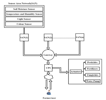Figure 1: Architecture for Monitoring Agro Systems

Figure 2: Representing Energy Efficient Algorithm in a Sensor Area Network (SAN 1)

4. Proposed Energy Efficient Algorithm

The proposed algorithm uses energy efficiently in agricultural applications to elongate the sensor nodes life time. The agro devices’ dormant mode will be synchronized and controlled by the proposed algorithm based on the change of day/night. This algorithm doesn’t depend on the marketable power supplies so it will guarantee a sustainable environment.  The battery drainage issue will be solved to some extent which will enable a sustainable power system. The proposed energy efficient algorithm is dependent on the load scheduling technique and solar energy. There are two other methods for powering the system either by using battery only or by using battery along with load scheduling.

The proposed algorithm is compared with these two methods. In the first method as shown in Figure 3, there is no enough power for supplying the loads as they are active for only five consecutive hours. In the second method, load scheduling technique is used which saves more power therefore the loads are active for longer time as shown in Figure 3. However. The problem of battery drainage still exists and the battery needs to be replaced but it is not easy to replace it in agro-applications. Replacing the battery is not necessary in the proposed algorithm as the solar panel is used during day to recharge the battery. The loads are supplied by the battery only during night. The solar panel is used to supply the loads during day therefore the battery state of charging is maintained for longer time in the proposed algorithm as shown in Figure 3. As a result of using the proposed algorithm, the life time of the sensor nodes is increased due to the increase of the battery life time.

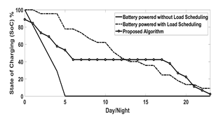Figure 3: State of Charging versus Day/Night for The Two Power Methods Compared with The Proposed Algorithm.

The two main parameters used in the proposed algorithm are the availability of power and the criticality index of the load. The first parameter is represented as solar irradiance or State of Charging (SoC) of the battery. The second parameter indicates whether the load is critical or not to operate in the non-scheduled time. Based on these two main parameters, the agricultural ecosystems loads are transferred to on or off state. Intelligent load Scheduling and solar power are combined in this algorithm to efficiently implement the system using IoT.

Figure 4 represents a flow chart for a combined energy efficient technique using intelligent load scheduling and solar energy. The algorithm initially checks the capacity of solar power during day to decide whether to activate or deactivate the load. It is proven in the simulation that the idle duration varies based on the availability of solar power. For example, when the solar irradiance is reduced from 1000 W/m²   to 500 W/m², the idle duration is increased by Δt. The battery is the source of power during night and it takes the lead in the absence of the sun to supply all the needed loads.

The loads are transferred to on or off state based on their criticality index as the loads are classified according to priority. The loads with high and medium priority are activated if SoC of battery is more than or equal to 75% and the unnecessary loads are deactivated. According to the availability of power, the loads’ idle time is tuned and calculated.  By time, the idle duration increases as a function of the battery drainage. If SoC is below 40%, the load with high priority is activated and the load with medium priority is deactivated and the idle duration increases based on the drainage rate of the battery. The inactive loads can be transferred to on state if needed during night based on user request.

The idle duration levels during day and night are shown in Table 1. The first level is selected during day as it is devoted for the dynamic solar irradiance scenario in which it varies during day hours from 100 W/m² to 1000 W/m². The other levels are devoted for the battery SoC variations. According to the availability of power, the idle duration for each load changes by Δt. Table 1 shows different scenarios where the idle duration level for each load changes by Δt and according to this change, the power gain is calculated for each load. The power gain shows the state of the consumed power at the current level compared to the previous level. As shown in Figure 5, the power gain increases as the Δt increases.

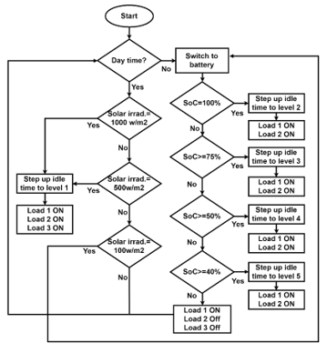Figure 4: The Flow Chart Illustrates That the Decision of Activating or Deactivating the Loads is Taken After Checking State of Charging (SoC) of The Battery and the Availability of Light.

Table 1:  Representing the Power Gain and The Changes in Idle Time for Different Scenarios

Level	Scenario	Load Priority	Active Hours	Δt           (Hours)	Power Gain (dBm)
1	Dynamic Irradiance	High	11	10	46.48
		Medium	5	5	45.22
		Low	4	4	44.25
2	100%	High	12	1	36.47
		Medium	6	1	38.23
		Low	0	4	44.25
3	≥75%	High	10	2	39.48
		Medium	4	2	41.25
		Low	0	0	0
4	≥50%	High	6	4	42.49
		Medium	2	2	41.25
		Low	0	0	0
5	≥40 %	High	4	2	39.48
		Medium	1	1	38.23
		Low	0	0	0
6	<40 %	High	1	3	41.25
		Medium	0	1	38.23
		Low	0	0	0

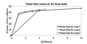Figure 5: Power Gain versus The Change in Idle Time (Δt) for The Three Loads

It is very essential to choose the optimum sleep time (T_s) that will not affect the system operation. There are three significant parameters that must be taken into consideration while choosing T_s,  State of Charging (SoC), Load current (I_L) , and Load index (η). The load index (η) ranges from 0.1 to 1. The value 1 indicates high priority, 0.5 indicates medium priority and 0.1 indicates low priority. The SoC is the difference between the battery rated capacity (C_rated) and the used capacity by loads (C_used) divided by the battery rated capacity. SoC can be calculated using (2):

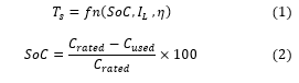Figure 6 represents the charging stage of the battery which shows that the battery state of charging is increasing with time. As a result the sleep duration for the loads is decreasing due to the increase of the amount of power available in the battery. Therefore the sleep duration is inversely proportional to the SoC as shown in Figure 7. Figure 8 shows that the increase in load current results in a decrease in the battery state of charging.

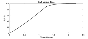Figure 6:   SoC Represented in a Charging Stage versus Time

Figure 7: Sleep Duration versus Time

Figure 8:  State of Charging at Different Load Currents versus Time

The active duration for each load depends on the maximum current consumed by the loads (I_Lmax), the current consumed by load 1 (I_L1) and the load index (η). Equation (3) is used to calculate the active duration for each load then calculate the sleep duration using (4). The active and sleep durations for the three loads are shown in Figure 9 and 10. Figure 11 represents the sleep duration for each load versus the battery SoC.

Figure 9: Active Duration for Three Loads versus State of Charging (SoC)

Figure 10: Sleep Duration for Three Loads versus State of Charging (SoC)

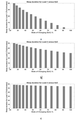Figure 11:  Sleep Duration for Each Load versus State of Charging (SoC)

Figure 12:  Energy Consumed by Each Load versus Sleep duration for Each Load

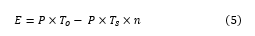
The energy consumed by each load for a uniform sleep duration depends on the power consumed by the load (P), the operating time (T_o), Sleep time for each load (T_s) and the number of sleep durations (n). The energy consumed by each load is calculated using (5). As shown in Figure 12, the energy consumed by each load decreases by increasing the sleep duration.

5. Simulation Model Results

An agro environment is simulated on a Matlab Model that is designed using one node consisting of battery, three loads and solar panel. The designed model is used to test the algorithm by testing it at different scenarios that are shown in Tables 2 and 3. The solar irradiance and the state of charging must be checked first to enable the model to select the optimal scenario based on these two parameters. This scenario selection will guarantee the efficient use of energy which will increase the battery life time. The current and power of the solar panel is affected by solar irradiance so a decrease in solar irradiance causes a decrease in the current and power as shown in Figure 13. Low solar irradiance occurs as a result of the small amount of solar energy absorbed by the solar panel which results in a decrease in power and current. Due to the change in climatic conditions as shown in Table 2, solar irradiance changes. The solar power is affected by these changes and it will have an effect during day on deciding whether to switch loads on or off.

Figure 13:  Power and Current at Different Solar Irradiances

Table 2 and 3 show the different scenarios that are designed depending on the battery state of charging and the changes in solar irradiance during day. The loads are activated or deactivated based on the availability of energy provided by battery or solar panel. High priority load is represented as load 1, medium priority load is represented as load 2 and low priority load is represented as load 3. Table 2 shows the four scenarios that are used usually during night. These scenarios are designed depending on the state of charging of the battery. During night, load 1 and load 2 are active for specific hours based on priority while load 3 is deactivated.

Table 2:  Represents Different Scenarios of Load Scheduling During Night

Scenario #	Scenario Description	SoC (%)	hrs	Load Scheduling Scenarios		Load Active hours (hrs)
				Priority	Status
1	Fully charged	100	12	High	On	12
				Medium	On	6
				Low	Off	0
2	Partially charged	75	12	High	On	10
				Medium	On	4
				Low	Off	0
3	Half charged	50	12	High	On	6
				Medium	On	2
				Low	Off	0
4	Battery draining	<40		High	On	1
				Medium	Off	0
				Low	Off	0

Figure 14 shows the battery state of charging as it decreases with time. It is essential to monitor the battery state in order to select the best scenario for supplying loads during night based on amount of power remained.

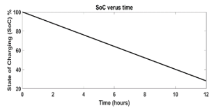Figure 14: Battery State of Charging versus Time

The solar irradiance is divided into two types static and dynamic. Static solar irradiance is represented in the first three scenarios that are shown in Table 3. These scenarios are designed for various cases that might occur during day in case of static solar irradiance. The duration is constant for the first three scenarios as it is estimated to be 12 hours.

In case the solar irradiance is dynamic during day, this is represented in the fourth scenario shown in Table 3. Scenario 4 is designed due to the change of solar irradiance during day hours. The values of solar irradiance in the previous scenarios might happen in one scenario at different hours. The first scenario in Table 2 and the fourth scenario in Table 3 are simulated and shown in Figure 16 and 17.

Figure 15 shows the changes in solar irradiance during day while during night the loads are supplied by the battery. These variations have an effect on solar power provided to the loads which will decide the status of the load.

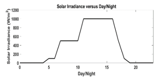Figure 15:  Solar Irradiance versus Day /Night

Table 3: Represents Different Scenarios of Load Scheduling During Day

Scenario #	Scenario Description	Climatic Conditions	Solar Irradiance	hrs	Load Scheduling Scenarios		Load Active hours (hrs)
					Priority	Status
1	Static Irradiance	Direct sunlight	1000 W/m2	12	High	On	12
					Medium	On	10
					Low	On	8
2	Static Irradiance	Cloudy sunlight	500   W/m2	12	High	On	6
					Medium	On	4
					Low	On	2
3	Static Irradiance	Very cloudy	100   W/m2	12	Powered by Battery Only
4	Dynamic Irradiance	Clear direct sunlight	1000 W/m2	6	High	On	6
					Medium	On	3
					Low	On	3
		Cloudy sunlight	500   W/m2	5	High	On	5
					Medium	On	2
					Low	On	1
		Very cloudy	100    W/m2	3	Powered by Battery Only

The loads’ status shown in Figure 16 has an effect on its total consumed energy as it changes due to the change in loads’ status during day and night. The compensation factor (CF) is shown in Figure 22 as it is calculated for the eight scenarios. It is defined as the ratio between the loads’ consumed energy and the energy supplied. During day hours, the solar irradiance changes and at noon, it reaches the maximum point. The solar power at the maximum point will be enough to supply all the loads as shown in Table 3 for specific hours.

Figure 16:  Loads (On/Off Status) versus Day/Night (Scenario 1 in Table 2 and Scenario 4 in Table 3)

      Figure 16(a) shows the status of load 1 during day and night. During day hours, load 1 is supplied by solar and in this case the load is active. While during night, it is supplied by the battery.

Figure 16(b) shows the status of load 2, it is activated during day for only 5 hours. Load 2 is activated during night for 6 hours. Figure 16(c) shows the status of load 3, it is activated during day for only 4 hours and it is deactivated at night.

The calculation of load‘s consumed energy is according to the status of loads shown in Figure 16.  The supplied energy either by solar or battery is efficiently consumed using the load scheduling scenarios to provide a sustainable system as shown in Figure 17.

Figure 17: Total Energy Consumed versus Day/Night (Scenario 1 in Table 2 and Scenario 4 in Table 3)

      Scenario 2 in Table 2 along with scenario 4 in Table 3 are tested and shown in Figure 18 and 19.  Figure 18 shows the loads on/off status during day and night. The total consumed energy by the loads is calculated based on the status of loads as shown in Figure 19.

Figure 18(a) shows that during day hours, load 1 is activated as the power is provided by solar in this case while at night, the load is still activated and supplied by the battery. Figure 18(b) shows that during day, load 2 is activated for only 5 hours and it is activated for 4 hours at night. Figure 18(c) shows that during day, load 3 is activated for only 4 hours but at night it is deactivated.

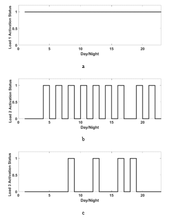Figure 18:  Loads (On/Off Status) versus Day/Night (Scenario 2 in Table 2 and Scenario 4 in Table 3)

The efficient usage of energy during day and night will provide a sustainable system. The total consumed energy by the loads during day and night in accordance to the loads’ status is shown in Figure 19.

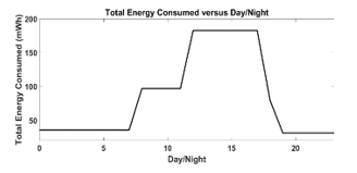Figure 19: Total Energy Consumed versus Day/Night (Scenario 2 in Table 2 and Scenario 4 in Table 3)

Scenario 3 in Table 2 along with scenario 4 in Table 3 are simulated and represented in Figure 20 and 21. Figure 20 shows the status of the loads which indicates whether it is on or off during day and night. Figure 21 shows the total consumed energy by the loads during day and night based on the status of the loads.

      Figure 20(a) shows the status of load 1 during day and night. During day, load 1 is activated by solar power for only 10 hours. During night, it is activated for only 6 hours as it is supplied by the battery.  Figure 20(b) shows the status of load 2 during day and night. During day, load 2 is activated for only 5 hours and at night it is inactive. Figure 20(c) shows the status of load 3 during day and night. During day, load 3 is activated for only 4 hours and at night it is inactive. The supplied energy is consumed efficiently by the loads using the designed scenarios of load scheduling. The total consumed energy by the loads during day and night is shown in Figure 21.

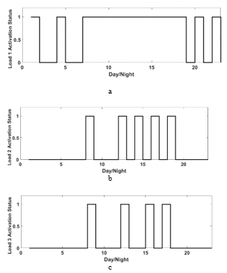Figure 20:  Loads (On/Off Status) versus Day/Night (Scenario 3 in Table 2 and Scenario 4 in Table 3)

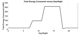Figure 21: Total Energy Consumed versus Day/Night (Scenario 3 in Table 2 and Scenario 4 in Table 3)

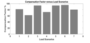Figure 22:  Compensation Factor (CF) versus Load Scenarios

Figure 22 represents the compensation factor (CF) which is calculated for all the designed scenarios. It is the consumed energy by the loads relative to the energy supplied by solar or battery. The compensation factor (CF) is used to show whether there will be an amount of remaining energy that can be used for battery charging or all the supplied energy is fully consumed by the loads.

6. Discussion

      The proposed algorithm was simulated and its results are shown in Table 4. The main source that was used for supplying power to the loads during day is the solar panel. During day, there are four designed scenarios for load scheduling. In scenario 1, the three loads will be activated based on priority for a certain time and the energy consumed by the loads is 671.94 mWh at 1000 W/m².  When the solar irradiance changes to 500 W/m², the solar power in this case isn’t enough for supplying all loads so scenario 1 isn’t suitable for this case as the loads activation period must be reduced.

In this case, scenario 2 is chosen as load 1 (highest priority) is activated for 6 hours while load 2 (medium priority) is activated for 4 hours and load 3 (lowest priority) is activated for 2 hours. In this scenario, the energy consumed by the loads is 184.32 mWh, the battery can be recharged during day using the remaining solar power. At 100 W/m², scenario 3 is selected as the loads are supplied by the battery because the solar power is not enough for supplying the loads in this case. The three solar irradiances 1000, 500 and 100 W/m²   can vary during day so they are combined and represented in scenario 4.  In scenario 4, the solar irradiance is 100 W/m²   for 3 hours, 500 W/m²   for 5 hours, and 1000 W/m² for 6 hours.

Table 4:  Simulation Results for Energy Efficient Algorithm

Power Source	Scenario #	Power (mw)			Energy (mwh) for different scenarios	CF %
		Load 1	Load 2	Load 3
Solar	1	4.62	1.65	75	671.94	81.26
	2	4.62	1.65	75	184.32	61.64
	3	4.62	1.65	75
	4	4.62	1.65	75	359.07	71.77
		4.62	1.65	75
		4.62	1.65	75
Battery	1	4.62	1.65	75	65.34	93.33
	2	4.62	1.65	75	52.8	94.73
	3	4.62	1.65	75	31.02	79.93
	4	4.62	1.65	75

During night, the algorithm was simulated by using the battery as the main source of power for supplying the loads. There are also four designed scenarios for load scheduling at night. In scenario 1, the loads are supplied by a fully charged battery so load 1 is activated for 12 hours while load 2 is activated for 6 hours as it is active for 1 hour every 2 hours and load 3 is inactive. In scenario 2, the battery SoC is 75 % so load 1 is active for 12 hours, load 2 is active for 4 hours as it is active for 1 hour every 3 hours and load 3 is inactive. Load 3 can be activated based on the user demand or it remains inactive till the availability of light. In scenario 3, the battery SoC is 50% so load 1 is active for 6 hours as it is active for 1 hour every 2 hours while load 2 is active for 2 hours as it is active for 1 hour every 6 hours and load 3 is inactive. In scenario 4, the battery SoC is below 40% so load 1 is active for 1 hour while load 2 and 3 are switched off till the availability of light in order for the loads to be powered by the solar and for the battery to be recharged. The proposed algorithm guarantees the efficient usage of energy by using the designed scenarios for load scheduling during day and night. It provides a sustainable system as it avoids the drainage of the battery which will prolong the system life time.

7. Conclusion

As a conclusion, it is essential to monitor plants’ performance as it helps in increasing and saving the agricultural production. Monitoring the performance of plants is facilitated using IoT technology as it uses wireless sensors that enables the plants to talk and express its requirements. Energy optimization is a major challenge that faces IoT. In agriculture, wireless sensors are utilized in remote areas therefore they consume high energy for continuous operation. An energy efficient technique was proposed in this paper to avoid battery drainage in order to guarantee system sustainability and continuous operation. Solar power and intelligent load scheduling are combined in the proposed algorithm. The results showed that the system operation adapts to the availability of power represented as solar irradiance or battery SoC. It operates using solar panels during day based on solar irradiance but during night, it depends on the battery SoC.  During day and night, intelligent load scheduling based on priority is applied to ensure continuous operation. The proposed algorithm elongates the sensors’ batteries life time as it efficiently uses energy to ensure the system sustainability. The proposed algorithm enhanced the battery life time by 79.2 %.

1. S.S. Abou Emira, K.Y. Youssef, M. Abouelatta, “Adaptive power system for IoT-based smart agriculture applications,” in ICENCO 2019 – 2019 15th International Computer Engineering Conference: Utilizing Machine Intelligence for a Better World, IEEE: 126–131, 2019, doi:10.1109/ICENCO48310.2019.9027393.
2. S.S. Sarmila, S.R. Ishwarya, N.B. Harshini, C.R. Arati, “Smart farming: Sensing technologies,” in Proceedings of the 2nd International Conference on Computing Methodologies and Communication, ICCMC 2018, 149–155, 2018, doi:10.1109/ICCMC.2018.8487571.
3. S. Rawal, “IOT based Smart Irrigation System,” International Journal of Computer Applications, 159(8), 7–11, 2017, doi:10.5120/ijca2017913001.
4. S. Naveen, S. Hegde, “Study of IoT: Understanding IoT Architecture, Applications, Issues and Challenges,” in 1st International Conference on Innovations in Computing & Networking (ICICN16), CSE, RRCE, 477–482, 2016.
5. D.A. Vyas, D. Bhatt, D. Jha, “IoT: Trends , Challenges and Future Scope,” International Journal of Computer Science & Communication, 7(1), 186–197, 2016, doi:10.090592/IJCSC.2016.028.
6. S. Sadasivam, V. Vadhri, Smart Plant Monitoring System, Informatik, Technische Universitat Darmstadt, Darmastatd, 2015.
7. D. Markovic, R. Koprivica, U. Pesovic, S. Randic, “Application of IoT in monitoring and controlling agricultural production,” Acta Agriculturae Serbica, 20(40), 145–153, 2015, doi:10.5937/aaser1540145m.
8. K.Y. Chan, H.J. Phoon, C.P. Ooi, W.L. Pang, S.K. Wong, “Power management of a wireless sensor node with solar energy harvesting technology,” Microelectronics International, 29(2), 76–82, 2012, doi:10.1108/13565361211237662.
9. H.M. Jawad, R. Nordin, S.K. Gharghan, A.M. Jawad, M. Ismail, M.J. Abu-Alshaeer, “Power reduction with sleep/wake on redundant data (SWORD) in a wireless sensor network for energy-efficient precision agriculture,” Sensors (Switzerland), 18(10), 3450–3475, 2018, doi:10.3390/s18103450.
10. H. Swalehe, P.V. Chombo, B. Marungsri, “Appliance scheduling for optimal load management in smart home integrated with renewable energy by using whale optimization algorithm,” GMSARN International Journal, 12(2), 65–75, 2018.
11. X. Liu, L. Ivanescu, R. Kang, M. Maier, “Real-time household load priority scheduling algorithm based on prediction of renewable source availability,” IEEE Transactions on Consumer Electronics, 58(2), 318–326, 2012, doi:10.1109/TCE.2012.6227429.
12. S. Trivedi, K. Parkh, K. Agrawal, “Load Scheduling for Smart Energy Mangement in Buildings with Renewable Power Generation,” International Journal of Engineering Research And, 6(03), 322–326, 2017, doi:10.17577/ijertv6is030349.
13. M.R. Mohd Kassim, I. Mat, A.N. Harun, “Wireless sensor network in precision agriculture application,” in 2014 International Conference on Computer, Information and Telecommunication Systems, CITS 2014, 1–5, 2014, doi:10.1109/CITS.2014.6878963.

(Click Here)