1.Introduction

The successful of the development of numerical techniques for boundary value problems has been growing rapidly in the past few decades. Many researchers give more attention to this problem numerically and show the capability of their numerical techniques in solving this problem especially TPBVPs; due to its application, this problem can be found in science, engineering and physics fields including optimal control, beam deflection and heat flow [1-4]. In initial works on obtaining the numerical solutions of TPBVPs, many authors attempted to achieve higher accuracy by using the various numerical methods. It was done either by suggesting the families of spline methods for solving second-order two-point boundary value problem, see in [5-9]. The basic approach of these methods is dividing the interval into subinterval and at the same time, the construction of spline, B-spline and extended B-spline in each subinterval considered. For achieving better accuracy, these methods are required to solve a system of equations. Another numerical method is to solve TPBVPs by developing the innovative method based on the Galerkin method see in [10-12]. Numerous numerical methods are used to solve the boundary value problems related TPBVPs for obtaining the approximation equation can be seen in [13-17].

Besides of using the above numerical methods to solve the proposed problem (1) as stated in the first paragraph, many studies were also introduced via the use of the concept of finite difference method (FDM). As a result, several numerical discretization schemes mainly in a family of the finite difference schemes have been proposed to form a new finite difference discretization scheme. For example, the standard finite difference [18], Chebyshev finite difference [19] and Rational Finite Difference [20] are imposed for solving TPBVPs. Clearly, the development of Chebyshev finite difference and Rational Finite Difference schemes has been encouraged by the combination of the standard finite difference concept together with the Chebyshev and rational approximation functions respectively.  In conjunction with these combinations, the author in [20] also introduced a new finite difference scheme via the combination of exponential approximations and finite difference discretization schemes which is known as exponential finite difference discretization schemes to show its capability for solving TPBVPs [21].

Apart from the use of Chebyshev, rational and exponential approximation functions as mentioned in the previous second paragraph, this paper attempts to investigate the feasibility of the Redlich-Kister polynomial as a numerical method for solving TPBVPs. Based on the previous studies on the application of the Redlich-Kister polynomial, the findings have pointed out that various types of Redlich-Kister polynomial functions have successfully been used to develop the appropriate mathematical models in physics and chemistry fields [22-24].  In addition to these functions, only one study has been explored to investigate the application of the Redlich-Kister approximation function in the numerical analysis particularly on constructing the mathematical model. For instance, in [25], the authors investigated the construction of two mathematical models based on the piecewise third-order Redlich-Kister polynomial model and the piecewise first-order polynomial model respectively to show the relationship of the number of iterations for Gauss-Seidel towards its corresponding grid size. The findings of their work concluded that the results of the piecewise third-order Redlich-Kister polynomial model gave highly accurate solutions as compared with the first-order polynomial solution. Inspired by the high accuracy of the Redlich-Kister (RK) function based on high-order approximation function, we present a feasibility study of two newly established Redlich-Kister Finite Difference (RKFD) discretization schemes for solving TPBVPs.

In order to solve the proposed problem, firstly, the RKFD discretization scheme will be used to discretize TPBVPs to form the RKFD approximation equation. After that, the approximate equation was obtained will lead us to construct a linear system. Since the generated linear system has a large and sparse matrix, the use of iterative methods is the best linear solver [26-28]. For instance, the implementation of the point iteration family namely SOR [29], AOR [30] and KSOR [31] can be used to solve this linear system. In addition to this point iteration family, Evans [32] introduced the Explicit Group (EG) iterative method which is faster than the Gauss-Seidel (GS) iterative method to get the numerical solution of this linear system. Despite the speed up the convergence rate for Explicit Group (EG) iteration, many researchers also developed new variants of the EG iteration family such as 9-Point EG [33], EGSOR [34], EDGSOR [35] and MEGSOR [36] in which all these block iterations have significantly reduced their convergence rate. Therefore, further discussion of this paper focuses on investigating the efficiency of the 4EGKSOR iterative method which is inspired by the paper research [37] and apply together with the newly established RKFD discretization scheme for solving the system of Redlich-Kister approximation equations. The formulation of the 4EGKSOR iterative method can be established via the combination of the EG and KSOR iterative methods.

Before applying and investigating the performance of this 4EGKSOR method, we need to do the process of discretization and let us consider the general equation for TPBVPs, which are given as follows

with the Dirichlet conditions,

2. Redlich Kister Finite Difference Approximation Equation

The previous section has mentioned that the use of the RK function to introduce two newly established RKFD discretization schemes for approximating the proposed problem (1). To start the discretization process, firstly let us consider the RK approximation function of order n as follows

where are the unknown parameters to be determined.

Figure 1: Distribution of grid network considered.

To facilitate us in discussing the use of this approximation function, let us construct the distribution of uniformly node points as indicated in Figure 1. Based on Figure 1, let us consider the first three RK functions that need to consider the number of node points as shown in Figure 2.

Figure 2: The path for T₁, T₂ and ₃.

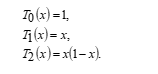
Then to derive the new second-order RKFD approximation equation, let us consider in equation (2) and applying the concept in Figure 2, the second-order RK approximation function can be written as

where the first three RK functions are defined as

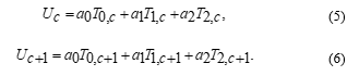
Referring to Figure 1, let us define the node points, where  donates the uniform step size. Then  and represent the approximation value of functions,  and By considering any group of three node points, and  for equation (3), we have the following equations

After that, the expression of three parameters in equation (3) can be determined by solving the equations (4), (5) and (6) via a matrix approach. With these three parameters, we rewrite the second-order RK approximation function,   in equation (3) in which it can be shown as follows

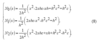
where the second-order RKFD shape functions, are defined respectively as

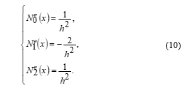
     Then the first and second derivative of these RK shape functions can be shown as

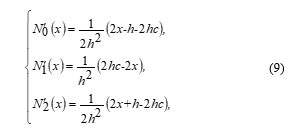and

     Then, by applying the first derivative concept into the function (7) with respect to it can be shown that the second-order RKFD discretization scheme of the first derivative of the function, is given as

and for the second derivative of the function  with respect to  can be approximated by

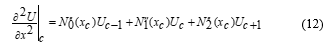where represent the approximation solution of function Clearly, equations (11) and (12) are known as two newly established Redlich-Kister finite difference discretization schemes.

From the proposed problem (1), it needs to be rewritten in the discrete form at a node point,  and then we get

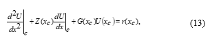Then by considering both equations (11) and (12) and substitute them into equation (13), it can be pointed out that the newly established RKFD approximation equation of TPBVPs can be formulated as follows

where

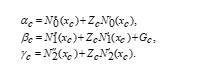and

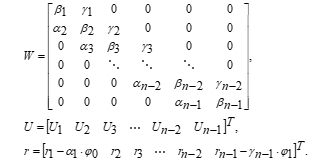
     Referring to the RKFD approximation equation (14) and considering   it is obvious that we can construct a generated linear system with its large-scale and sparse coefficient matrix  as follows

where

3. Derivation of 4EGKSOR Iterative Method

Since the characteristics of the coefficient matrix of the linear system (15) are large-scale and sparse, the family of iterative methods can be chosen to be the best linear solver as stated in the first section. To solve this linear system, the Kaudd Successive Over Relaxation (KSOR) iterative method was developed by [38] as one of more efficient point iterative methods by using one weighted parameter which is used to speed up its convergence rate and show to be more economical computationally than the Gauss-Seidel (GS) iterative method. Due to the advantage of lower computational complexity, we establish the formulation of the Four-Point Explicit Group Kaudd Successive Over Relaxation (4EGKSOR) iterative method, which is a combination between a standard Kaudd Successive Over Relaxation (KSOR) iterative method and Explicit Group approach by using the newly established RKFD approximation equation (14).  To derive the formulation of 4EGKSOR, let us consider the grid network in Figure 1 and a group of block node points concept in Figure 3. Figure 3 illustrates the finite grid network of the RKFD approximation equation where block approach has been done until iteration convergence is achieved.

Figure 3: Distribution of grid network for 4EGKSOR method.

Before discussing more details on the formulation of the 4EGKSOR method, let us consider the coefficient matrix (15) being defined as

where is diagonal matrix, and are strictly lower and upper matrices of the generated linear system (15) . Then, the large-scale and sparse linear system (15) becomes

 In drive to achieve the linear system (17) based on the point iteration approach, the implementation of the KSOR method over the linear system can be stated in matrix form as follows [31,39]

where indicates the current value of at the   iteration.

Again, imposing the KSOR method (18) can also be rewritten in the point iteration approach as follows

for whereas the optimum value of the different value subject to the size value of The range value of is given [31] by

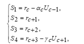
By using the same steps to obtain equation (19), let us begin to introduce the KSOR block iteration approach. To start this discussion, let us consider again a sequence of a group of four and three node points in Figure 3. As we can see that two types of blocks were used to form during the implementation of the 4EGKSOR iteration. Firstly, the four-point block iteration is applied for the completed group of four and three point block is imposed into the ungrouped case. Referring to equation (15), the 4EGKSOR iterative method is defined as [37]

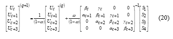where

Meanwhile, for the ungrouped case has been applied for only one group of three points block is shown as follows

where

Thus, Algorithm 1 describes a summary of the 4EGKSOR iterative method, which has been implemented for solving the proposed problem (1).

Algorithm 1:4EGKSOR iteration

i.          Set the initial value

ii.          Calculate the coefficient matrix,

iii.          Calculate the vector,

iv.          For  calculate the equation (20).

v.          For  calculate the equation (21).

vi.          Check the convergence test, If yes, go to step (vii). Otherwise, go back to step (iv).

vii.          Display approximate solution.

4. Numerical Problem and Discussion

In this section, we investigate the feasibility of the 4EGKSOR iterative method for solving three examples of one-dimensional TPBVPs and then compared with GS and KSOR methods which are set up as a benchmarking for this study. All the results that have been obtained by imposing these three methods considered into these three examples are analyzed based on three comparison parameters such as the number of iterations (Iter), execution time (Time) in seconds and maximum norm (MaxNorm) at five different sizes, In this study, we also set up the value of tolerance error, for all grid sizes are considered.

Example 1 [40]

Consider one-dimensional TPBVPs as

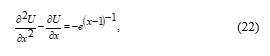The analytical solution of problem (22) is

Example 2 [41]

Consider one-dimensional TPBVPs

The analytical solution of problem (23) is

Example 3 [42]

Consider one-dimensional TPBVPs

The analytical solution of problem (24) is

All results of GS, KSOR and 4EGKSOR iterative methods in solving these three examples are stated in Tables 1, 2 and 3 and illustrated in Figure 4, 5, and 6 respectively. Table 4 shows that the reduction percentage of KSOR and 4EGKSOR iterative methods which compared with GS method for three examples considered.

Table 1: Numerical results based on comparison criteria considered for Problem 1.

n	Method	Iter	Time	MaxNorm
256	GS	82043.0	7.92	4.0343e-07
	KSOR	769.0	0.75	2.4866e-07
	4EGKSOR	364.0	0.17	2.3889e-07
512	GS	292276.0	16.23	2.5291e-06
	KSOR	1526.0	1.67	6.7370e-08
	4EGKSOR	759.0	0.44	8.0806e-08
1024	GS	1025489.0	76.67	1.0346e-05
	KSOR	2853.0	3.19	2.5732e-08
	4EGKSOR	1295.0	0.78	4.7925e-08
2048	GS	3527433.0	409.03	4.1443e-05
	KSOR	5792.0	6.63	1.7614e-08
	4EGKSOR	2545.0	1.50	5.9857e-08
4096	GS	11811519.0	2359.09	1.6579e-04
	KSOR	10221.0	10.41	9.8302e-08
	4EGKSOR	5369.0	3.13	7.2651e-08

Table 2: Numerical results based on comparison criteria considered for Problem 2.

n	Method	Iter	Time	MaxNorm
256	GS	92156.0	19.79	9.0029e-07
	KSOR	796.0	0.81	1.5811e-06
	4EGKSOR	414.0	0.30	1.5584e-06
512	GS	329819.0	58.89	2.4116e-06
	KSOR	1559.0	1.69	3.7928e-07
	4EGKSOR	756.0	0.39	4.0320e-07
1024	GS	1164082.0	257.58	1.1096e-05
	KSOR	3073.0	3.56	1.0466e-07
	4EGKSOR	1450.0	0.82	6.2177e-08
2048	GS	4035615.0	1345.67	4.4746e-05
	KSOR	6145.0	7.18	3.8252e-08
	4EGKSOR	2826.0	1.71	4.3353e-08
4096	GS	13659733.0	2913.87	1.7907e-04
	KSOR	11571.0	11.03	5.2215e-08
	4EGKSOR	5181.0	3.06	1.0216e-07

Table 3: Numerical results based on comparison criteria considered for Problem 3.

n	Method	Iter	Time	MaxNorm
256	GS	89973.0	19.88	5.4091e-07
	KSOR	782.0	0.37	1.9062e-07
	4EGKSOR	381.0	0.17	2.0338e-07
512	GS	318924.0	60.80	2.9059e-06
	KSOR	1537.0	0.89	5.2948e-08
	4EGKSOR	724.0	0.40	2.5886e-08
1024	GS	1111808.0	256.86	1.1810e-05
	KSOR	3057.0	1.82	1.5546e-08
	4EGKSOR	1387.0	0.79	6.1722e-08
2048	GS	3791677.0	1260.25	4.7285e-05
	KSOR	5734.0	3.43	2.5772e-08
	4EGKSOR	2753.0	1.75	8.8766e-08
4096	GS	12544476.0	2681.69	1.8915e-04
	KSOR	10655.0	5.78	1.0642e-07
	4EGKSOR	5463.0	3.21	1.1934e-07

Table 4: Reduction percentage for the KSOR and 4EGKSOR in term of the iteration and time.

N	Method	Iter	MaxNorm
Problem 1	Iter	99.06-99.84	99.56-99.95
	Time	89.71-99.56	97.29-99.87
Problem 2	Iter	99.14-99.92	99.55-99.96
	Time	95.91-99.62	98.48-99.89
Problem 3	Iter	99.13-99.92	99.57-99.96
	Time	98.13-99.92	99.14-99.96

Figure 4: Comparison of three iterative methods based on error over the solution domain of Problem 1 at n = 4096.

All results are presented in Tables 1 to 4, the KSOR method gives reduced iteration and speeds up its execution time as compared with GS iterative method. Then, in terms of a reduction percentage, the KSOR iteration in Example 1 has significantly reduced number of iterations approximately by 99.06-99.84% and speed up by 89.71-99.56%. For Examples 2 and 3 also give the pattern as same as Example 1 in which KSOR iteration is better than GS iteration. However, the 4EGKSOR iteration gives tremendously improved either in the number of iterations or execution time which are 99.56-99.95% and 97.29-99.87% for Example 1, 99.55-99.96% and 98.48-99.89% for Example 2 and 99.57-99.96% and 99.14-99.96% for Example 3 respectively. In conclusion, it shows that the KSOR iteration has greatly reduced its number of iterations and execution time as compared to the GS iteration. It means that the 4EGKSOR iteration has the least amount compared to GS and KSOR iterations in terms of the number of iterations and execution time. In addition to these findings, for the maximum norm, KSOR and 4EGKSOR iterative methods show a good agreement and become close to their analytical solution compared to GS iterative method, see in Figures 4, 5 and 6.

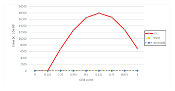Figure 5: Comparison of three iterative methods based on error over the solution domain of Problem 2 at n = 4096.

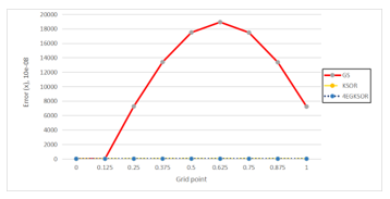Figure 6: Comparison of three iterative methods based on error over the solution domain of Problem 3 at n = 4096.

5. Conclusions

The formulation of GS, KSOR and 4EGKSOR iterative methods have been successfully derived by using two newly established RKFD discretization schemes for solving TPBVPs. Then, the generated large-scale and sparse linear system based on two newly established RKFD approximation equations have been solved by using three iterative methods in which all results were recorded. Based on the implementation of these three iterative methods, the 4EGKSOR iterative method has tremendously reduced the iteration and Time as compared with GS and KSOR methods. Therefore, the combination of the KSOR block technique with the standard EG iterative method can reduce iteration and Time compared to the KSOR point approach. For further study, this paper can be extended to perform the use of the newly established RKFD discretization scheme for solving the multi-dimensional boundary value problems by using the two-step iteration family [43,44], and the half-sweep [45,46] and quarter-sweep [47,48] iteration families.

Acknowledgment

The authors would like to express sincere gratitude to Universiti Malaysia Sabah for funding this research under UMSGreat research grant for postgraduate student: GUG0494-1/2020.

1. J. Aarao, B. H. Bradshaw-Hajek, S. J. Miklavcic, and D. A. Ward, “The extended domain eigen-function method for solving elliptic boundary value problems with annular domains.” Journal of Physics A: Mathematical and Theoretical, 43, 185-202, 2010, doi:10.1088/1751-8113/43/18/185202.
2. T. N. Robertson, “The linear two-point boundary value problem on an infinite interval.” Mathematics Of Computation, 25(115), 475-481, 1971, doi:10.1090/s0025-5718-1971-0303742-1.
3. Y. M. Wang, and B. Y. Guo, “Fourth-order compact finite difference method for fourth-order nonlinear elliptic boundary value problems.” Journal of Computational and Applied Mathematics, 221(1), 76-97, 2008, doi:10.1016/j.cam.2007.10.007.
4. Y. Gupta, “A numerical algorithm for solution of boundary value problems with applications.” International Journal of Computer Applications, 40(8), 2012, doi:10.5120/4988-7252.
5. C. Nazan, and C. Hikmet, “B-spline methods for solving linear system of second order boundary value problems.” Computers and Mathematics with Application, 57(5), 757-762, 2008, doi:10.1016/j.camwa.2008.09.033.
6. B. H. Lin, W. H. Huan, and C. Yanpeng, “Polynomial spline approach for solving second-order boundary-value problems with neumann conditions.” Applied Mathematics and Computation, 32, 6872-6882, 2011, doi:10.1016/j.amc.2011.01.047.
7. N. N. A. Hamid, A. A. Majid, and A. I. M. Ismail, “Extended cubic B-spline method for linear two-point boundary value problems.” Sains Malaysiana, 40(11), 1285-1290, 2011,doi:10.5281/zenodo.107900.
8. J. Rashidinia, and S. Sharifi, “B-spline method for two-point boundary value problems.” International Journal of Mathematical Modelling and Computations, 5(2), 111-125, 2015, doi:10.1016/j.cam.2010.10.031.
9. M. N. Suardi, N. Z. F. M. Radzuan, and J. Sulaiman, “Cubic b-spline solution for two-point boundary value problem with aor iterative method.” Journal of Phiysics: Conference Series, 890, 012015, 2017, doi:10.1088/1742-6596/890/1/012015.
10. M. El-Gamel, “Comparision of the solution obtained by Adomian decomposition and wavelet-galerkin methods of boundary-value problems.” Applied Mathematics and Computation, 186(1), 652-664, 2007, doi:10.1016/j.amc.2006.08.010.
11. A. Mohsen, and M. E. Gamel, “On the galerkin and collocation methods for two point boundary value problems using sinc bases.” Computer and Mathematics with Applications, 56, 930-941, 2008, doi:10.1016/j.camwa.2008.01.023.
12. M. M. Rahman, M. A. Hossen, M. N. Islam, and M. S. Ali, “Numerical solutions of second order boundary value problems by Galerkin method with Hermite polynomials.” Annals of Pure and Applied Mathematics, 1(2), 138-148, 2012, doi:10.1.1.684.13.
13. B. Jang, “Two-point boundary value problems by extended adomian decomposition method.” Computational and Applied Mathematics, 219(1), 253-262, 2007, doi:10.1016/j.cam.2007.07.036.
14. S. M. Roberts, and J. S. Shipman, “Continuation in shooting methods for two-point boundary value problems.” Journal of mathematical analysis and applications, 18(1), 45-58, 1967, doi:10.1016/0022-247x(67)90181-3 .
15. C. F. Price, “An offset vector iteration method for solving two-point boundary-value problems.” The Computer Journal, 11(2), 220-228, 1968, doi:10.1093/comjnl/11.2.220.
16. R. P. Agarwal, “On the method of complementary functions for nonlinear boundary-value problems.” Journal of Optimization Theory and Applications, 36(1), 139-144, 1982, doi:10.1007/bf00934344 .
17. Q. Fang, T. Tsuchiya, and T. Yamamoto, “Finite difference, finite element and finite volume methods applied to two-point boundary value problems.” Journal of Computational and Applied Mathematics, 139(1), 9-19, 2002, doi:10.1016/s0377-0427(01)00392-2 .
18. M. M. Chawla, and C. P. Katti, “Finite difference methods for two-point boundary value problems involving high order differential equations.” BIT Numerical Mathematics, 19(1), 27-33, 1979, doi:10.1007/bf01931218 .
19. E. M. Elbarbary, and M. El-Kady, “Chebyshev finite difference approximation for the boundary value problems.” Applied Mathematics and Computation, 139(2-3), 513-523, 2003, doi:10.1016/s0096-3003(02)00214-x .
20. P. K. Pandey, “Rational finite difference approximation of high order accuracy for nonlinear two point boundary value problems.” Sains Malaysiana, 43(7), 1105-1108, 2014.
21. P. K. Pandey, “Solving two point boundary value problems for ordinary differential equations using exponential finite difference method.” Boletim da Sociedade Paranaense de Matemática, 34(1), 45-52, 2016, doi:10.5269/bspm.v34i1.22424 .
22. S. Babu, R. Trabelsi, T. Srinivasa Krishna, N. Ouerfelli, and A. Toumi, “Reduced redlich–kister functions and interaction studies of dehpa+ petrofin binary mixtures at 298.15 k.” Physics and Chemistry of Liquids, 57(4), 536-546, 2019, doi:10.1080/00319104.2018.1496437 .
23. A. Gayathri, T. Venugopal, and K. Venkatramanan, “Redlich-kister coefficients on the analysis of physico-chemical characteristics of functional polymers.” Materials Today: Proceedings, 17, 2083-2087, 2019, doi:10.1016/j.matpr.2019.06.257.
24. N. P. Komninos, and E. D. Rogdakis, “Geometric investigation of the three-coefficient redlich-kister expansion global phase diagram for binary mixtures.” Fluid Phase Equilibria, 112728, 2020, doi:10.1016/j.fluid.2020.112728 .
25. M. K. Hasan, J. Sulaiman, S. Ahmad, M. Othman, and S. A. Abdul Karim, “Approximation of iteration number for gauss-seidel using redlich-kister polynomial.” American Journal of Applied Sciences, 7, 956-962, 2010, doi:10.3844/ajassp.2010.969.975 .
26. D. M. Young, Iterative Solution Of Large Linear Systems. London: Academic Press, 1971.
27. W. Hackbusch, Iterative Solution of Large Sparse Systems of Equations. Springer-Verlag, 1995.
28. Y. Saad, Iterative Methods for Sparse Linear Systems, International Thomas Publishing, 1996..
29. R. Rahman, N. A. M. Ali, J. Sulaiman, and F. A. Muhiddin, “Caputo’s finite difference solution of fractional two-point boundary value problems using SOR iteration.” In AIP Conference Proceedings, 2013, 1, 2018, doi:10.1063/1.5054233 .
30. A. Sunarto, J. Sulaiman, and A. Saudi, “Implicit finite difference solution for time-fractional diffusion equations using AOR method.” In Journal of Physics: Conference Series, 495, 1, 2014, doi:10.1088/1742-6596/495/1/012032 .
31. N. Z. F. M. Radzuan, M. N. Suardi, and J. Sulaiman, “KSOR iterative method with quadrature scheme for solving system of Fredholm integral equations of second kind.” Journal of Fundamental and Applied Sciences, 9(5S), 609-623, 2017, doi:10.4314/jfas.v9i5s.43 .
32. D. J. Evans, “Group explicit iterative methods for solving large linear systems.” International Journal of Computer Mathematics, 17(1), 81-108, 1985, doi:10.1080/00207168508803452 .
33. A. Saudi, and J. Sulaiman, “Robot path planning using four point-explicit group via nine-point laplacian (4EG9L) iterative method.” Procedia Engineering, 41, 182-188, 2012, doi:10.1016/j.proeng.2012.07.160 .
34. K. Ghazali, J. Sulaiman, Y. Dasril, and D. Gabda, “Application of Newton-4EGSOR Iteration for solving large scale unconstrained optimization problems with a tridiagonal hessian matrix.” In Computational Science and Technology (pp. 401-411). Springer, Singapore, 2019, doi:10.1007/978-981-13-2622-6_39 .
35. A. Saudi, and J. Sulaiman, “Path Planning Simulation using Harmonic Potential Fields through Four Point-EDGSOR Method via 9-Point Laplacian.” Jurnal Teknologi, 78(8-2), 2016, doi:10.11113/jt.v78.9537.
36. J. Sulaiman, M. K. Hasan, M. Othman, and S. A. A. Karimd, “MEGSOR iterative method for the triangle element solution of 2D Poisson equations.” Procedia Computer Science, 1(1), 377-385, 2010, doi:10.1016/j.procs.2010.04.041 .
37. F. A. Muhiddin, J. Sulaiman, and A. Sunarto, “Implementation of the 4EGKSOR for Solving One-Dimensional Time-Fractional Parabolic Equations with Grünwald Implicit Difference Scheme.” In Computational Science and Technology (pp. 511-520). Springer, Singapore, 2020, doi:10.1007/978-981-15-0058-9-49.
38. I. K. Youssef and A. A. Taha, “On modified successive overrelaxation method.” Applied Mathematics and Computation, 219, 4601-4613, 2013, doi:10.1016/j.amc.2012.10.071 .
39. I. Youssef, “On the successive overrelaxation method.” Journal of Mathematics and Statistics, 8(2), 176-184,2012, doi:103844/jmssp.2012.176.184.
40. H. N. Caglar, S. H. Caglar, and K. Elfaituri, “B-spline interpolation compared with finite difference, finite element and finite volume methods which applied to two point boundary value problems.” Applied Mathematics and Computation, 175(1), 72-79, 2006, doi:10.1016/j.amc.2005.07.019.
41. Y. Li, J. A. Enszer, and M. A. Stadtherr, “Enclosing all solutions of two-point boundary value problems for odes.” Computer and Chemical Engineering, 32(8), 1714-1725, 2008, doi:10.1016/j.compchemeng.2007.08.013 .
42. M. A. Ramadan, I. F. Lashien, and W. K. Zahra, “Polynomial and nonpolynomial spline approaches to the numerical solution of second order boundary value problems.” Applied Mathematics and Computation, 184, 476-484, 2007, doi:10.1016/j.amc.2006.06.053 .
43. A. A. Dahalan, M. S. Muthuvalu, and J. Sulaiman, “Numerical solutions of two-point fuzzy boundary value problem using half-sweep alternating group explicit method.” American Institute of Physics, 1557(1), 103-107, 2013, doi:10.1063/1.4823884 .
44. A. A. Dahalan, J. Sulaiman, and M. S. Muthuvalu, “Performance of HSAGE method with Seikkala derivative for 2-D fuzzy Poisson equation.” Applied Mathematical Sciences, 8(17-20), 885-899, 2014, doi:10.12988/ams.2014.311665.
45. M. K. Hasan, J. Sulaiman, S. A. Abdul Karim, and M. Othman, “Development of some numerical methods applying complexity reduction approach for solving scientific problem.”, 2010.
46. A. Saudi, and J. Sulaiman, “Red-black strategy for mobile robot path planning.” In World Congress on Engineering 2012. July 4-6, 2012. London, UK, International Association of Engineers, 2182, 2215-2219, 2010.
47. N. I. M. Fauzi, and J. Sulaiman, “Quarter-Sweep Modified SOR iterative algorithm and cubic spline basis for the solution of second order two-point boundary value problems.” Journal of Applied Sciences (Faisalabad), 12(17), 1817-1824, 2012, doi:10.3923/jas.2012.1817.1824.
48. J. V. Lung, and J. Sulaiman, “On quarter-sweep finite difference scheme for one-dimensional porous medium equations.” International Journal of Applied Mathematics, 33(3), 439, 2020, doi:10.12732/ijam.v33i3.6.

(Click Here)

No. of Downloads Per Month

No. of Downloads Per Country