1. Introduction

Reducing water consumption is a fundamental constituent of water management, particularly in water-scarce areas. In many countries, irrigation water is one of the major contributors to water scarcity, and reducing irrigation water while increasing water efficiency is a way to overcome this issue. This work, which is an extension of the paper originally presented in 2019 8th International Conference on Modeling Simulation and Applied Optimization (ICMSAO) ‎[1], looks at different practices used to reduce the use of irrigation water and proposes the use of an advanced optimization technique as possible solution to the problem.

Different mulching practices, irrigation techniques and irrigation strategies can reduce water consumption in irrigation. Mulching refers to the practice of covering the soil with protective material to reduce evapotranspiration. Irrigation techniques (dripping, furrow, sprinkler etc.) refer to the way irrigation water is applied, which also affects evapotranspiration. Irrigation strategies refer to the timing and the amount to irrigation water provided to the crop. Irrigation scheduling, which refers to when and how much to irrigate, is a fundamental concept associated with irrigation strategies ‎[2], ‎[3]. Although mulching practices, irrigation techniques and irrigation strategies are all important tools, in ‎[2] it is found that for optimal results, the irrigation strategy should be improved first, followed by mulching practices and the irrigation technique. Therefore, in the present study we will focus on irrigation strategies and, in particular, on water-efficient irrigation technology.

Technological developments include automated irrigation systems, that irrigate at set times and for a certain amount of time. Although these automated techniques present advantages in terms of increased water efficiency and reduced farmers’intervention, the performances of these open loop control systems in terms of water consumption are not yet optimal. The main reason of their unsatisfactory performance is that they can cause under- or over-watering, since weather and crop conditions are not taken into account. This of course can lead to spoiled crop and water wastage.

Greater expectation is placed on technologies which include sensors and closed-loop watering systems ‎[4]-‎[6]. The simplest approach uses sensors in an on/off control scheme, where irrigation is turned on or off depending on the reading of a moisture sensor above or below set values.

More complex control strategies, which often are model-based, have been described in different papers ‎[7]-[10]. In general, model-based control strategies require models of the soil moisture dynamics including variables such as climatological data, crop water needs, water saturation etc. ‎[7], ‎[8]. Among such advanced control strategies is Model Predictive Control (MPC), as proposed in the research described in ‎[9] and ‎[10]. The models presented in ‎[9] and ‎[10] are based on the water balance equation, which requires measuring or estimating the initial soil moisture, rainfall, water capacity of the soil and evapotranspiration (ET). From these measurements, the water balance equation gives an estimation of the soil moisture. In these papers, the MPC algorithm is formulated as an optimization problem, which reduces set point tracking errors.

Similarly to the work presented in ‎[9] and ‎[10], our work describes the development of a soil moisture dynamic model and its application in a predictive control setting. However, the predictive control strategy here proposed is based on Economic Model Predictive Control (EMPC), which aims at maximizing the economic performance of the irrigation system rather than reducing tracking errors. Constraints in the optimization problem are used to guarantee that optimal soil moisture is obtained. Moreover, in the present study the soil moisture model is based on atmospheric conditions of the Kingdom of Bahrain ‎[11].

The remainder of this paper is organized as follows. Section 2 describes the derivation of the soil moisture model based on the water balance equation and the measurement of meteorological data of the Kingdom of Bahrain. Section 3 describe the principles of MPC and presents EMPC as a special case of the MPC policy. In Section 4 the outcomes of employing the EMCP are shown and comparisons are drawn with On-off and PID automated irrigation systems. Finally, conclusion and recommendations are included in Section 5.

2. System Identification

This section presents the grey-box modeling of the soil moisture dynamics using difference equations. Grey-box modeling is a method for identifying the system’s dynamics that uses measurement obtained from experimental data combined with physical knowledge of the system. For parameters estimation, state space models are often used, where the state, input and output of the system are related by difference equations.

2.1. Physical Modelling

2.1.1. Water-balance equation

The model developed here is based on the water-balance equation represented graphically in Figure 1 ‎[9], ‎[10]:

where k is the sampling time, M is the moisture of the soil, IR is the irrigation water, RAIN is the precipitation, CR is the capillary rise, ET_c is the crop evapotranspiration, DP is the deep percolation and RO is the water runoff.

Equation (1) expresses the variation in soil moisture as the difference between the water influx (capillary rise, precipitation and irrigation) and the water losses (evaporation, transpiration, water runoff and deep percolation) ‎[10].

Geomorphological and meteorological data of the Kingdom of Bahrain show a generally flat land and very scarce precipitations. Therefore, it is reasonable to assume that water runoff, precipitation, and capillary rise are negligible. Under these assumptions, (1) can be reduced to:

Equation (2) reduces the dependency of soil moisture to three variables: irrigation, evapotranspiration and deep percolation.

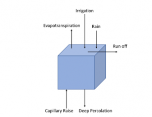
Figure 1: Water Balance Model

2.2. Evapotranspiration Estimation

Evapotranspiration is defined as the movement of water from the soil and the crop into the atmosphere. Many factors influence evapotranspiration rate, such as crop type and growth stage, weather factors (air temperature, wind, humidity etc.), environmental conditions (e.g. soil salinity) and land management (use of fertilizers and pesticides, etc.) ‎[12].

Different approaches exist to estimate evapotranspiration ‎[13]. In the present study, the FAO Blaney-Criddle estimation approach has been used. Despite being a simpler method compared to others, it has been proven to be satisfactory under a variety of weather conditions ‎[14], ‎[15].

Using this method, the actual evapotranspiration ET_c is estimated for a particular type of crop C as:

In (3), the crop coefficient K_c depends on the crop type and the growth stage of the crop. ET_o is the estimation of the evapotranspiration from the reference crop with hypothetical qualities (actively growing green grass of 8–15 cm height). In the present study, ET_o is assumed to be affected by climatic parameters, according to the following empirical FAO Blaney –Criddle equation:

where T_mean is the average daily temperature [°C] and p is the average annual percentage of daytime.

2.3. Deep Percolation

Deep percolation (DP) is a hydrologic process, where water penetrates below the roots of the crop. The quantity of percolation during irrigation depends on the characteristics of the soil as well as the soil humidity.

In the present study, DP is assumed to be directly proportional to M with proportionality constant K_p: when M increases, DP increases due to differential pressure [16]. This is expressed by the following equation:

In (5), K_p is a constant that depends on the type of soil (sandy, clay, silt, loamy, etc)

Substituting (3) and (5) in (2) we get a difference equation which leads to a model of the water balance dynamic in the form:

where K_s=1-K_p.

2.4. Model Structure

Equation (6) gives a mathematical model which contains two parameters, K_s and K_c. In our work, these parameters are unknown, meaning that the value of crop coefficient and the type of soil used in our experiment are unknown. Therefore, a gray-box system identification process, which uses a the first principles model of the system and data coming from direct system measurements, was used to estimate the values of the unknown parameters.

The linear difference equation (6) can be re-written in the form of a discrete state space model as:

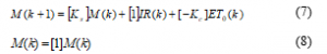
where M(k), IR(k), ET₀(k) are the state vector, the input signal, and the disturbance of the system.

The state-space model (7) and (8) presents two parameters, K_s and K_c, that need to be estimated from measured data.

2.5. Parameters Estimation

Parameter estimation was carried out using Matlab System Identification Toolbox R2018a, which provides a tool for deriving mathematical models of dynamic systems given measured input-output data. The toolbox was used to estimate the values of K_s and K_c, through a gray-box model estimation process.

Figure 2 shows the process of model identification.

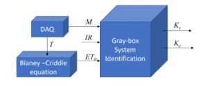
Figure 2: Model Identification Process

A set of measurements (see Figure 3), called identification data, was collected using a data acquisition system implemented on an Arduino Uno microcontroller board.

The experimental setup consists of a temperature sensor LM35, and a soil moisture sensor FC-28. The temperature sensor outputs a voltage which is directly proportional to the instantaneous temperature. The soil moisture sensor measures the volumetric soil moisture as a function of electric conductivity in the soil. In our experiment, the position of the soil moisture sensor was fixed at 10 cm depth. The sensor was calibrated by taking two measures; one with the soil entirely wet and one with the soil entirely dry. The moisture was expressed in percentage, with the values of the measurements mapped from 0 (dry soil) to 100 (soaked soil).

Figure 3: Identification Data

For our experiments, the soil moisture M and the temperature T near the moisture sensor were synchronously measured every hour over a period of two days. The irrigation IR was modeled as a pulse signal, since it provides a great amount of water but for a limited time ‎[10].

The Blaney-Cradle equation block in Figure 2 estimates ET_o using (4). In our experiment, the value of the variable p in (4) was substituted by the actual percentage of daytime for the time of the year in which the experiment was conducted. In the same way, the variable T_mean was substituted by the actual temperature T measured at time k.

2.6. Model Validation

To validate the model obtained in the previous section the output of the simulated model was compared with measured data.

For this purpose, another set of input data was measured and then inputted to the derived model of the system. The input data set used in the validation is shown in Figure 4.

Figure 4: Validation Data

Figure 5 shows the difference between the output of the model and the measured soil moisture. The plots show a good agreement between simulated and measured outputs, with negligible time delay between the irrigation event and the change in soil moisture dynamics.

A further comparison between simulated and measured outputs to verify the reliability of the identified model was done calculating the Mean Absolute Error (MAE) as follows:

where  is the difference between the predicted and the measured output value and T=48 is the total number of samples. The obtained MAE value of 2% is considered an indication of a valid model.

Figure 5: Measured and Simulated Soil Moisture

3. Economic MPC

3.1. EMPC Basic Concepts

The term Predictive Control refers to a control design method characterized by [17]:

• use of a model to forecast the system output at future time instants (prediction horizon);
• computation of an input control sequence that optimizes a given objective function;
• receding horizon strategy, where the input control sequence is computed by taking into account the predicted outputs, but only the first control signal of the sequence is applied to the system.

The different algorithms which belongs to the Predictive Control group present differences in terms of the chosen system models (impulse, step, state-space, CARIMA, fuzzy models, etc.), disturbance (constant, decaying, filtered white noise etc.) and in the cost-function to be minimised.

A general MPC mathematical formulation is given by the following optimization problem ‎[18]:

where the variables x ∈ Rⁿ and u ∈ R^m denote the state and control action at the instant k and H_c denotes the control horizon. The notation , with k ∈ Z, indicates the estimation of the future variables based on the measurements at current time instant k.

Traditional MPC controllers minimize a quadratic cost function which tracks output and manipulated variable references.

The general prediction model can be expressed by the discrete equation:

where the predicted states depend on the future states and control actions from instant k to instant k+H_p.

The minimization problem is usually subject to a set of constraints which have to be satisfied over the predictive horizon. These constraints are due to physical or operational limitations of the real system and they take the general form:

At each time instant, MPC measures or estimates current state x_k and predicts the system state evolution over the prediction horizon H_p using the current state and the model of the system.

The optimal control sequence over the control horizon H_c is found solving the minimization problem (10). Only the first control action is applied to the system, and the remaining results are discarded.

In absence of disturbances and plant-model mismatch, the optimization problem could be solved as an open-loop problem, and the input sequence found at k=0 could be applied to the system for all k≥0. In a more realistic scenario, the behavior of the real system differs from the predicted model output. To cater for this mismatch, the optimal control problem is solved again at the next sampling time. Using the state measurement/estimation at time k+1, the cycle of prediction and optimization is repeated, moving the horizon forward (Figure 6).

Figure 6: Receding Horizon

In recent years, the EMPC approach has been proposed with successful applications in various fields ‎[19].

Contrary to traditional MPC, EMPC is employed to maximize profitability, rather than minimize tracking errors. This can be done by defining a cost function that, directly or indirectly, measures the process economics ‎[20]. The formulation of cost function depends on the particular applications, such as the operating profit, production rates, product selectivity, and product yield. In EMPC the cost function, as well as the plant dynamics and the constraints can be linear or nonlinear. Therefore, generic performance cost functions and nonlinear optimization algorithms are used to solve the minimization problem. The structure of the basic EMPC algorithm is shown in Figure 7.

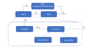
Figure 7: Basic EMPC Structure

3.2. EMPC Problem Formulation

In our work, we utilize an EMPC approach to minimize water consumption while maintaining the soil moisture close to an optimum value. We consider a linear economic stage cost function; additionally, both plant dynamics and constraints are linear. Because of this, our formulation of the EMPC problem is linear. The fundamental steps of the devised EMPC algorithm are the following:

• At the time k, measure M(k) and compute the optimal control sequence by solving a stochastic optimization problem over the control horizon N_c.
• Apply only the first computed value IR(k/k) as input to the system.
• At the time k+1, measure M(k+1) and repeat the optimization.

At each time instant k, a vector  of the moisture predicted values is computed, using the model given by (7) and (8):

The stochastic optimization problem becomes deterministic if we assume that ET_o does not change over the prediction horizon N_p., i.e.:

where ET_o(k) is calculated using (4) and the current measured temperature T(k).

Let’s define the future control signals as the vector:

The purpose of the designed control system is to obtain optimal economic performance. The following stage cost is assumed to reflect the nominal economic cost of irrigating the system over one sampling period, that is:

The cost function does not consider the cost of operating the valves or the cost of pumping water, since their minimization is not considered an objective in the present study.

The resulting optimization problem adopted in our EMPC controller formulation is:

In addition to the stage cost, the objective function contains the terms  which represent soft economic constraints.

The minimization problem (21) is subject to:

The value M_opt represents the soil moisture that should be kept constant for optimal operating conditions. The variable v(k) is a slack variable that is introduced to allow for small variation of the soil moisture M(k) around the optimal value. That is, we nominally want to satisfy M(k)=M_opt, and when these constraints are violated, an additional cost  is paid, weighted by the penalty parameter ρ. The choice of the parameter ρ is critical; when it is chosen too small, the value of the soil moisture might be far from the optimal one; when it is chosen too big, we might incur into infeasibility issues.

4. Simulation Results

The performances of PID controller, On-off controller and the proposed EMPC are compared. Not surprisingly, the behavior of the three control techniques is very different, as it can be observed in Figure 8 and Figure 9.

The On-off controller uses the measurement from a moisture sensor to switch the irrigation pump on or off based on whether the measurement is below or above maximum and minimum limits. The output from the device is either 100% on or off, with no middle state. Figure 8 shows the outcome using the On-off controller. In this example, the soil moisture minimum and maximum levels are fixed at 50% and 70%. As expected, the output presents a variation of the moisture level (overshoot) around the optimal value of 65%. Reducing the thresholds could help improving the underwatering issue, but it would imply a higher switching of the actuators and a persistent overwatering problem.

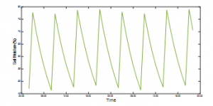
Figure 8: Soil Moisture with On-Off Controller

In Figure 9 the outcomes of the PID and EMPC approaches are shown. It can be noticed that the EMPC maintains the value of the soil moisture around the optimal value better that the PID controller in presence of disturbances, since it considers the effect of ET_o(k) on the moisture level over the prediction horizon.

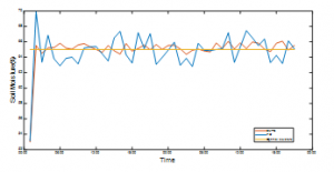
Figure 9: Soil Moisture Dynamics with EMP and PID Controllers

The three irrigation systems are also compared in terms of accumulated error, defined as:

where the error is the difference between the optimal soil moisture and the simulated soil moisture. The cumulative error gives an indication of the ability of the controller to keep the soil moisture close to the optimal value. As it can be seen in Figure 10, the EMPC has smaller cumulative error compared to the other irrigation methods.

The total water consumption over the 48 hours period is around 2400 ml for the On-off controller, 2160 ml for the PID based system and 2000 for the EMPC. Therefore, the EMPC yields a reduction of water consumption around 8% and 16% compared with the PID and On-off controllers, respectively, while keeping the soil moisture within optimal values.

The simulations demonstrate that the EMPC scheme applied to an irrigation system provides benefits compared to conventional irrigation methods, since it maintains the moisture level near the nominal optimum, while providing economic benefit.

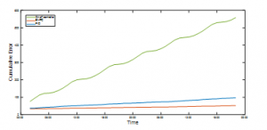
Figure 10: Cumulative Error for On-Off Controller, PID and EMPC

5. Conclusions

This work presents the process of developing an optimal controller regulating the time and amount of irrigation to maintain the soil moisture around an optimal level, while taking into account system constraints. The proposed control strategy, based on EMPC techniques, was implemented in MATLAB and results were compared with traditional irrigation methods based on PID and On-Off controllers. The results suggest that EMPC applied to irrigation systems can lead to increased efficiency and reduced water consumption.

Further improvement of this work would require a more accurate model of the system. A current limitation is given by the model developed, which can be improved by collecting sensors measurements over a sparse area and under different operating conditions, and using more complicated approaches to estimate ETo such as the FAO Penman Montheith technique.

Furthermore, developments on this work could explore the implementation of the proposed EMPC algorithm on hardware and evaluate the feasibility of such strategy in real time.

Conflict of Interest

The authors declare no conflict of interest.

1. L. Balbis, “Economic Model Predictive Control for Irrigation Systems,” in 2019 8th International Conference on Modeling Simulation and Applied Optimization (ICMSAO), Manama, Bahrain, 2019. https://doi.org/10.1109/ICMSAO.2019.8880332.
2. A. D. Chukalla, M. S. Krol, A. Y. Hoekstra, “Marginal cost curves for water footprint reduction in irrigated agriculture: guiding a cost-effective reduction of crop water consumption to a permit or benchmark level” Hydrol. Earth Syst. Sci., 21(7), 3507–3524, 2017. https://doi.org/10.5194/hess-21-3507-2017, 2017.
3. A. D. Chukalla, M. S. Krol, A. Y. Hoekstra, “Green and blue water footprint reduction in irrigated agriculture: effect of irrigation techniques, irrigation strategies and mulching” Hydrol. Earth Syst. Sci., 19(12), 4877–4891, 2015. https://doi.org/10.5194/hess-19-4877- 2015.
4. R. Aqeel-ur, A.Z. Abbasi, S. N. Islam, Z. A. Shaikh, “A Review of Wireless Sensors and Networks Applications in Agriculture” Computer Standards & Interfaces, 36, 263-270, 2014. https://doi.org/10.1016/j.csi.2011.03.004.
5. P. Alagupandi, R. Ramesh and S. Gayathri, “Smart irrigation system for outdoor environment using Tiny OS,” in 2014 International Conference on Computation of Power, Energy, Information and Communication (ICCPEIC), Chennai, India, 2014. https://doi.org/10.1109/ICCPEIC.2014.6915348.
6. M.W. van Iersel, M. Chappell, J. D. Lea-Cox, “Sensors for Improved in Efficiency of Irrigation in Greenhouse and Nursery Production”, HortTechnology, 23(6), 735-746, 2013. https://doi.org/10.21273/HORTTECH.23.6.735
7. S. Kulkarni, “Innovative Technologies for Water Saving in Irrigated Agriculture” International Journal of Water Resources and Arid Environments, 1(3), 226-231, 2011. ISSN 2079-7079
8. J. B. Million, T. H. Yeager, J. P. Albano, “Evapotranspiration-based irrigation scheduling for container-grown Viburnum odoratissimum” HortScience, 45, 1741-1746, 2010. https://doi.org/10.21273/HORTSCI.45.11.1741
9. S. K. Saleem, D. K. Delgoda, S. K. Ooi, K. B. Dassanayake, L. Liu, M. N. Halgamuge, H. Malano, “ Model Predictive Control for Real-Time Irrigation Scheduling”, in 2013 4th IFAC Conference on Modelling and Control in Agriculture, Horticulture and Post Harvest Industry, Espoo, Finland, 2013. https://doi.org/10.3182/20130828-2-SF-3019.00062.
10. Lozoya C., Mendoza C., Mej L., Quintana J., Mendoza G., Bustillos M., Arras O., Sol L., “Model Predictive Control for Closed-Loop Irrigation”, in 2014 19th World Congress, Cape Town, South Africa, 2014. https://doi.org/10.3182/20140824-6-ZA-1003.02067.
11. L. Balbis and A. Jassim, “Dynamic Model of Soil Moisture for Smart Irrigation Systems,” in 2018 International Conference on Innovation and Intelligence for Informatics, Computing, and Technologies (3ICT), Sakhier, Bahrain, 2018. https://doi: 10.1109/3ICT.2018.8855748.
12. M. Todorovic, Crop evapotranspiration, in book: Water Encyclopedia: Surface and Agricultural Water, John Wiley & Sons Publisher, 2005.
13. R.G. Allen, L.S. Pereira, D. Raes, M. Smith, “Crop evapotranspiration: guidelines for computing crop water requirements” in FAO Irrigation and Drainage, FAO, Rome, Italy ,1998.
14. H. R. Fooladmand, “Evaluation of Blaney-Criddle equation for estimating evapotranspiration in south of Iran” in African Journal of Agricultural Research. 6(13), pp. 3103-3109, 2011.
15. O. E. Mohawesh, “Spatio-temporal calibration of Blaney-Criddle equation in arid and semiarid environment” in Water Resour. Manage., 24(10), 2187-2201, 2010. https://doi.org/10.1007/s11269-009-9546-7
16. S.K. Ooi, I. Mareels, N. Cooley, G. Dunn, G. Thoms, “A Systems Engineering Approach to Viticulture On-Farm Irrigation” in 2018 17th World Congress. Seoul, Korea, 2008. https://doi.org/10.3182/20080706-5-KR-1001.01618
17. E.F. Camacho, C. Bordons Introduction to Model Predictive Control, in book: Model Predictive Control. Advanced Textbooks in Control and Signal Processing, Springer, 2007.
18. J. M. Maciejowski, Predictive Control with Constraints, Prentice Hall, 2002.
19. T. Tran, K. Ling, J. M. Maciejowski, “Economic Model Predictive Control – A Review”, in 2014 31st International Symposium on Automation and Robotics in Construction and Mining, ISARC, Sydney, Australia, 2014. https://doi.org/10.3182/20080706-5-KR-1001.01618.
20. J. B. Rawlings, D. Angeli, C. N. Bates, “Fundamentals of economic model predictive control” in 2012 51st IEEE Conference on Decision and Control (CDC), Maui, Hawaii, USA, 2012. https://doi.org/10.1109/CDC.2012.6425822.

(Click Here)

(Click Here)