1. Introduction

International credit rating agencies note changes in exchange rates in relation to country credit ratings. The exchange rate represents the credit risk of the currency country viewed in the financial market. In [1], the author argued that the credit rating announcement by the credit rating agency has a significant impact on the exchange rate and its influence varies depending on emerging markets or developed countries. In [2], the author argued that the depreciation of the exchange rate is a negative factor for the financial system of the country. In [3], the author argued that large differences in interest rates between local and foreign currencies would increase dollar loans with low interest rates. In [4], the author that entities in East Asian countries use foreign currency loans to reduce borrowing costs. They argued that company selectively use foreign currency loans in consideration of low foreign currency borrowing interest rate benefits and foreign exchange hedge costs arising from foreign currency borrowing. As they argument, the mid- to long-term exchange outlook, adjusted according to interest rates, expected currency values, macro-economic variables, etc., are important for the parties to the foreign exchange transaction. Therefore, it is important to understand the mid- to long-term equilibrium relationship between each currency and with variables in each currency and international financial markets variables. However, the exchange rate is generally highly volatile in the short term, as the following arguments suggest. In [5], the author argued that the short-term exchange rate determinant model by macroeconomic variables is almost indescribable. In [6], the author argued that the empirical analysis of advanced countries’ currencies generally showed that the exchange rate was close to random walking, and that the won-dollar exchange rate was also random walking after the introduction of the floating exchange rate system in Korea.  In [7], the author argued that the sensitivity of the trade-in between the local currency and the foreign currency was greater under the floating exchange rate system. He argued that the floating exchange rate system also limits the ability of monetary authorities to carry out their own policies. The following studies have shown that emerging economies’ exchange rate-setting mechanisms and dollarization increase exchange rate volatility. In [8], the author studied the factors affecting the transactions of local and foreign currencies in emerging countries. He argued that the holding of the local currency or foreign currency depends on the level of interest rate on the foreign currency against the local currency and the expected depreciation of the local currency. Therefore, it was argued that the foreign currency trade was determined in accordance with reasonable expectations for the local currency and the foreign currency. In [9], the author argued that the dollarization generally increases in emerging economies. The dollarization is the use of the dollar (foreign currency) as a means of storing value instead of the local currency. The IMF defined the dollar phenomenon in emerging economies as the proportion of foreign currency deposits to broad cash. They used the dollarization level as the ratio of foreign currency deposits to M2. In [10], the author argued that the dollarization was a reasonable response from the investors to future uncertainties in emerging economies’ currencies. The dollarization also affects macroeconomic policies, foreign exchange risk management and exchange rate systems in emerging economies. In [11], the author  analyzed the Turkish currency using a VAR model. He argued that the dollarization is caused by instability in three macroeconomic variables: currency devaluation volatility, inflation volatility, and uncertainty forecast volatility. In [12], the author argued that the loss of confidence in economic management would reduce confidence in the local currency, thereby promoting the retention of foreign currencies.  Bank plays a pivotal role in developing emerging economies’ financial markets. Therefore, deepening the dollarization of banks’ assets and liabilities increases foreign currency exchange risk. He argued that the dollarization is not significant in countries where the financial industry has grown to a considerable level, but in countries with small financial industries, the dollarization is relatively large. The above studies suggest that the medium- to long-term relationship of exchange rates is important for parties to foreign exchange transactions. The demand and supply of foreign exchange trading arise from the import-export transactions of enterprises and the hedging of foreign exchange positions held and the capital markets transactions invested in stocks and bonds. Thus, long-term exchange rate relationships between currencies and key variables in the international financial market are important for businesses and investors. South-Korea, China and Japan are the top 10 global import-export trading partners. In addition, China and Japan are Korea’s largest export-import trading partners. The Korean won is a non-international currency, but the Chinese yuan and Japanese yen are SDR international currencies. As a non-international currency country, like most ASEAN countries, Korea has to do import-export transactions and capital market transactions with international currency countries. Therefore, it is an important issue for Korean import-export companies and pension fund investors to find out the long-term equilibrium relationship between the won dollar, the yuan, and the yen. Regarding exchange rate relationship between Korea, China and Japan. In [13], the author analyzed the non-international currency of the Won, the SDR international currency of the Yuan, and the Yen by applying CIP theory. The CIP theory is that there is an equilibrium relationship between the difference between the risk-free interest rates of the two currencies and the difference between the spot exchange rate and the forward exchange rate. Therefore, the country’s foreign exchange market maintains equilibrium relationship under the CIP theory. In general, international currency is not regulated and there are no restrictions to trade, so the CIP theory is established. Therefore, it is in principle impossible to trade risk-free arbitrage transaction that arises from the collapse of the CIP equilibrium relationship. They argued that the Yen, which is an international currency, is impossible for risk-free arbitrage transaction when considering the transaction cost. However, they argued that the Yuan, which is in the process of internationalization, and the Won, a non-international currency, imply arbitrage opportunities through SWAP transactions. In [14], the author used the VECM (Vector Error Correction Model) model to analyze the relationship between the country CDS Premiums of Korea, China and Japan, the exchange rate and the variables of the international financial market. They argued that while the country CDS Premiums of Korea and Japan were more closely related to the variables in the international financial market, the Chinese CDS Premiums had a weak relationship. In [15], the author used the VECM model to analyze the relationship between the international financial market variables and the spot exchange rate of Latin America and the country CDS Premium. He argued that although variables in the international financial market affect the spot exchange rate of Latin America countries, their impact varies from country to country.

This study analyzes the long-term equilibrium between the Korean won (onshore KRW and offshore Won-Dollar, herein “NDF KRW” where NDF is non deliverable forward), the Chinese yuan (onshore CNY and offshore CNH), and the Japanese yen JPY currency. And analyze the long-term equilibrium relationship between these currency and international financial market variables. The analysis results compared the characteristics of a total of five currency markets by dividing them into won (KRW and NDF KRW) and yuan (CNY and CNH) and yen JPY. This study can be differentiated from the existent researches based on the following; First, we have identified the long-term equilibrium relationship between the exchange rates of Korea won, China yuan, and Japan yen from the perspective of the international financial market. Second, the degree of integration with the international financial market was compared by comparing and analyzing the non-international currency, the won, the yuan and the yen, the international currency. Third, it was found that although the onshore and offshore yuan, which is being promoted for internationalization, is related to each other, there is a unique market characteristic that is distinguished from each other. Therefore, we have provided suggestions that company and international investors need yuan trading and yuan position management in consideration of the onshore and offshore yuan characteristics. The composition of the study is as follows; Chapter 1 describes the purpose and background of the research. Chapter 2 describes prior research and the variables used in analysis. Chapter 3 described the research model and the research methodology. Chapter 4 basic statistics, unit root test, and co-integration test of the analysis data. Chapter 5 presents the analysis results of the VECM model. Chapter 6 presents summaries and conclusions.

2. Previous research

2.1.  Dollarization

The dollarization is the use of the dollar (foreign currency) as a means of saving value instead of the local currency. However, there is no consensus as to the various hypotheses in previous studies about the dollar phenomenon and the cause of currency exchange trading. In [16], the author put together four types of research on the dollarization. First, the study that the dollarization increases when the policy and institutional financial system of the local currency finance is poor. In [17], the author and in [18], the author, and in [19], the author argued that financial markets are not naturally fostered, but are developed through the process of maintaining stable asset values through their own economic growth and continued policy and institutional legislation. In [20], the author and in [19], the author argued that the dollarization is caused by increased risk of default, expected currency devaluation and a lack of dollar liability mismatch information. They argued that market failures were caused by problems between financial industry instability and related legal systems, and the dollarization was also caused by poor policy results and financial market imperfections. Second, the study that devaluation of exchange rates causes capital outflow and aggravates effect on the financial statements of domestic companies. In [21], the author argued that, in the event of a crisis, a significant foreign debt repayment burden reduces aggregate demand and, therefore, further depreciation of the exchange rate occurs. They argued that this would worsen the company financial statements, making borrowing conditions more unfavorable. Third, the study of currency substitution in relation to the foreign currency hedging. If investors experience high inflation in assets held in their local currencies, they will replace their holdings with foreign currencies to maintain future asset values. In [22], the author outlined the theory of trade-in between two currencies. In [23], the author argued in empirical studies that inflation and currency exchange trading are strongly interrelated. In [24], the author argued that holding foreign currencies in emerging countries played a role in hedging macroeconomic risks in emerging country economies. He argued that if investors were concerned about inflation in their currencies, the demand for foreign currency holdings would continue to increase. Fourth, the study that portfolio investment manager will have foreign currency assets at an optimal rate to minimize the risk of their investment portfolios. In [25], the author used the Minimum Variance Portfolio (MVP) method to study with five Latin America countries. They confirmed that assets and liabilities of financial institutions are readjusted in accordance with changes in exchange rates to hedge the inflation. In [26], the author argued that the proportion of dollar assets in MVPs and the dollarization are positive correlations.

2.2. Internationalization of Yuan

In 2008, when the global financial crisis recurred, China proceeded the internationalization of the yuan, mainly in Hong Kong. The yuan was newly incorporated into the SDR international currency in October 2016. The internationalizing of the yuan was a major issue for non-international currency countries. It was because currency internationalization could be an alternative to addressing the exchange rate problems common to emerging Asian countries. However, it is necessary for companies and financial institutions in non-international currency countries that do business with China to understand the characteristics of the new international currency, the renminbi, to manage exchange rate risk. In [27], the author asserted four backgrounds for the internationalization of the yuan. First, currency internationalization brings about the development of the direct financial market, so it has the effect of increasing the efficiency of monetary policy. Second, internationalization of currency has a good function to reduce the difference in interest rates and exchange rates between currencies by enabling arbitrage trading when changes in monetary policy are expected. Third, it argued that currency internationalization could further expand the wealth effect of the currency by enticing investors in the international financial market. Fourth, it argued that currency internationalization could lead to an increase in yuan deposits abroad, thereby promoting the growth of the yuan’s international financial market. They summed up the requirements for the internationalization of the yuan as follows: The increase in China’s economic weight in the global economy, the convenient exchange function of the yuan, the development of financial market and the liberalization of the Chinese financial market, the development of the offshore yuan financial market and the expansion of the flexibility of the yuan exchange rate. In [28], the author and in [29], the author cited five common factors in currency internationalization: political, military power, economic scale, national financial soundness and financial market competitiveness. In [30], the author argued that the higher the proportion of GDP, which represents the size of the economy, and the higher the proportion of trade in the global economy, the higher the possibility of internationalization of currencies. Trade dependence and inflation, on the other hand, have a negative impact on currency internationalization. They also argued that the greater the share of the stock market, the higher the proportion of foreign bonds issued in the local currency, and the greater the financial opening, the greater the possibility of internationalization of currencies. In [31], the author studied the international demand for yuan as a means of value storage. He used the explanatory variables of existing research to analyze the yuan. He estimated that the demand for the yuan would be 1 to 2 percent of the global currency volume in 2015 and 3 to 8 percent in 2020. However, he said that if China actively liberalizes its capital market and opens up its financial markets, the yuan’s demand may rise more than expected as the yuan’s trading volume increases further in the international financial market. The previous study of internationalization of currency were summarized in Table 1 below.

Table 1: Pre-study of the internationalization of currency

		Description of variable
[Dependent variable]		Macroeconomic variables	Currency market variables	Financial market variables	Others
[Requirements to be used as foreign exchange reserves)	Chinn & Frankel	GDP portion Inflation rate	Exchange rate volatility depreciation rate	Foreign exchange transaction weight	time lag
	Chen et al	GDP portion, trade size portion, inflation rate	Exchange rate volatility		time lag
	Li Daokui et al	GDP portion Inflation rate	Exchange rate volatility depreciation rate
	Dae Won Oh	GDP portion, trade size portion, inflation rate	Exchange rate volatility	M2 / GDP Openness
[Currency internationalization requirements]	Seok Hyeon, Sang Heon Lee	GDP portion, Trade portion, Trade dependency, Inflation		Stock Market Openness	Financial openness
[RMB internationalization requirements]	Haihong & Yongding Yu	China’s Economy portion in the Global Market	Flexibility of exchange rate Convenient exchange	Financial liberalization Financial Market Development Offshore Market Development

In [32], the author analyzed the impact of the onshore Chinese yuan (CNY) on the offshore yuan (CNH) market in Hong Kong. According to their analysis, the change in the implied interest rate of the forward exchange rate in China immediately affects the renminbi forward exchange rate market in Hong Kong. In [33], the author analyzed the effect of interest rate volatility transferred from the Chinese market to the Hong Kong offshore renminbi market through a variance decomposition analysis. They argued that volatility was transferred from the Chinese market to the Hong Kong offshore market at an average of 60.9%. However, the effect of transferring volatility from the Hong Kong offshore market to the Chinese local market was insignificant at 13.8%. In [34],  the author analyzed the CNH and CNY markets from September 2010 to August 2013. They argued that CNY had a strong influence on CNH at the beginning of the analysis period, but argued that CNH’s influence on CNY increased in the later period. Therefore, they argued that CNH Hong Kong’s offshore yuan has predictive of CNY’s Chinese onshore yuan. In [35], the author studied the difference in price between CNH offshore renminbi and CNY onshore currency. They argued that the yuan liquidity and risk aversion of international financial market investors were the main causes of the price difference between CNY and CNH and incurring arbitrage trading. They argued that an increase in the inflow of yuan from the CNY onshore market to the CNH Hong Kong offshore market narrowed the CNH-CNY price difference, and thus the yuan exchange rate was adjusted based on the available liquidity in the market.

2.3. Analysis of variable

We describe the variables used in the fifteen VECM analysis models.  The first variable is the spot exchange rate. The exchange rate represents the credit risk of the currency country viewed in the financial market. In [2], the author argued that the depreciation of the exchange rate is a negative factor for the financial system of the country. In [36], the author argued that the depreciation of the exchange rate is a problem with the repayment of national debt.  In [37], the author argued that a sharp depreciation of the exchange rate lowers the value of the assets denominated in the local currency, resulting in a lack of foreign currency liquidity, which increases the occurrence of a default risk. The second variable is the 10-year US treasury interest rate. In [38], the author argued that the 10-year U.S. government bond interest rate is the benchmark for the level of interest expected by investors in international financial markets. In [39], the author argued that the determinants of investment capital flowing into emerging economies are largely attributable to supply factors, such as the level of U.S. treasury bond interest rates and preference for safe assets in the international financial market. It argued that a 50bp drops in interest rates on 10-year U.S. treasury bonds would increase the total inflow of capital into emerging economies by 13 percent. The third variable is credit risk spread. In [40], the author argued that credit risk spreads represent investors’ risk aversion and are explained by the spread difference between the 10-year U.S. treasury bond and credit risky bonds. In [41], the author argued that an increase in the hedge propensity of investors in the international financial market increases the credit risk spread, and that the credit risk spread is significant in explaining the EMBI index of emerging economies in 31 countries. Alsaka and ap Gwilym [1] argued that the announcement by the credit rating agency had a significant impact on exchange rate fluctuations. The fourth variable is the VIX index. VIX is Chicago Board Options Exchange Volatility Index and is a variability in S&P100 index option transactions. The index represents the level of hedge propensity among international financial market investors. The VIX index is to the extent that investors feel an event risk, and it is the risk compensation rate expected by investors who expect high returns in the international financial market. In [42], the author argued that the VIX index is an important explanatory variable that determines the rate of return on treasury bonds. In [43], the author argued that it is an important variable that explained the premium on government bonds in emerging countries. In [44], the author argued that VIX is an important variable that explains the CDS premium in Mexico, Turkey, and South Korea. In [38], the author argued that VIX is a factor that explains the premium on short-term government bonds. In [39], the author stated that the VIX index represents a preference for safe assets in the international financial market and that if the VIX index fall halves, total capital inflows from emerging economies would increase by 11%. The fifth variable is TED spread. TED spread is the difference between the 90-day yield on U.S. treasury bonds and the three-month interest rate on Euro-dollar Libor. TED spread represents the average level of risk felt by the counterparty in inter-bank money market transactions in the international financial market. Higher cross-bank counterparty risk burdens are considered to have increased TED spreads and increased hedging tendencies in the international financial market, worsening the funding situation. The change in TED spread implies changes in overall capital liquidity in the international financial market or changes in credit risk levels and bond rates. In [45], the author used the TED spread as a measure of the liquidity level of hedge funds. In [41], the author used TED spread as a measure of the liquidity of government-issued government bonds in the international financial market.

3. Research model

3.1. Research Analysis

In [46], the author analyzed the mid- to long-term relationship of the Turkish exchange rate using the VECM analysis model. He constructed a nominal exchange rate and market exchange rate model and analyzed it using the VECM analysis method. They argued that the market exchange rate model has better predictability of the future mid-term exchange rate than a random walk with and without drift. In [15], the author also used the VECM analysis methodology to analyze the relationship between the Latin America spot exchange rate and the international financial market variables (the 10-year US treasury interest rate, the credit risk spread between the AAA credit rating and the BBB credit rating, VIX index, TED spread). This study also analyzed the Granger Causality, the impulse response, and the variance decomposition analysis using VECM analysis methodology that studied the mid- to long-term exchange rate relationship. The analysis variables are Korea won onshore (KRW) and offshore won, NDF KRW (KWD1m), Chinese onshore (CNY) and offshore yuan (CNH), Japanese yen (JPY), 10-year US treasury bond interest rate (T10Y), credit risk spread, VIX index, TED spread. The Chinese yuan is analyzed by dividing the Chinese onshore yuan (CNY) market, the Hong Kong  offshore yuan (CNH) market, and the Seoul offshore yuan market (herein we refer as “CNK”). The Korean won is divided into the Seoul Foreign Exchange onshore (KRW) Market and the offshore NDF KRW market (KWD1M).  The offshore won NDF KRW, has the shortest maturity of one month’s forward rate. In [47], the author also analyzed the causal relationship between the spot exchange rate of the onshore won dollar and the offshore NDF KRW exchange rate (the same one-month forward rate). NDF KRW is a forward exchange contract in which only the difference between the forward exchange rate and the spot exchange rate is settled in dollars without having to exchange the principal of the contract at maturity. As of 2018, the Korea won’s NDF market is worth about $9.5 billion. The won is non-international, but there is no limit to profit-taking arbitrage transactions in which investors take advantage of the price gap between the Seoul foreign exchange KRW market and the Seoul bond market and the offshore NDF KRW market. Therefore, it is assumed that the won has become substantially and effectively internationalized. The Japanese yen is International currency. Therefore, it analyzes the yen traded in international financial markets as there is no distinction between onshore and offshore markets. A total of fifteen VECM analysis models are used to verify the long-term cointegration relationship between variables and apply the VECM analysis methodology only if the long-term cointegration relationship is valid at statistical confidence level. The data analysis period is from December 1, 2014, when the yuan (CNK) began trading on the Seoul foreign exchange market to November 30 2017. The daily average trading volume of the Seoul offshore yuan (CNK) currency market is $1.5 billion to $2 billion, ranking third to fourth among the global offshore yuan market. There is no restriction on transactions because CNK is the same offshore yuan as the Hong Kong offshore yuan (CNH). It also means that the cross rate between the currencies can also affect the won-dollar KRW exchange rate. Therefore, the data analysis period was set for three years from December 1, 2014 to November 30, 2017 to compare fifteen analysis models.

3.2. Analysis Model

This study first tests the long-term equilibrium relationship between the analysis variables using the cointegration analysis method proposed by [48] the author. In general, time series data are non-stationary and therefore have a unit root. However, if there is a stable linear combination between these variables, it can be considered that there is a cointegration relationship between the variables, so that a long-term, stationary relationship exists. Therefore, regression analysis can be used when a cointegration relationship is recognized even among unstable time series data. When the cointegration relationship is confirmed, the relationship between the variables is analyzed using the VECM model, which includes the error correction term (ECT) in the VAR model. The VECM model can measure the effect of the time lag between endogenous variables and analyze the long-term equilibrium relation between variables as well as the short-term dynamic relations simultaneously. Nevertheless, since the VAR model is not constrained, the results may vary depending on the variable settings. Therefore, this study performed Granger causality analysis in addition. The impulse response analysis was used to analyze how external impacts were transferred between variables. The study also add variance decomposition analysis to analyze the magnitude of the influence of unexpected impacts on variables. It is necessary to verify the cointegration relationship between research variables in order to apply the VECM analysis methodology. Thus, this study conducted Johansson’s cointegration analysis. The methods for verifying Johansen’s cointegration vector are trace (λ trace) and maximum eigenvalue (λ max) tests. The test statistic is as follows:

here, λ _i indicates the matrix eigenvalue and T is the observed number. The null hypothesis of λ trace is: “there is no cointegration”; if this is rejected, there exist at least r number of cointegration relations, and the variables become stable I (0) time series. Only after the cointegration verification is confirmed, the relationship between the endogenous variables is analyzed by applying the VECM analysis methodology. The cointegration test show the long-term equilibrium relationship between variables, but it does not suggest its direction. To overcome this problem, this study analysis the relationship between variables using VECM model. The use of the VECM model has the advantage of being able to identify both short- and long-term causal relationships, as it can identify not only the effects of the differential term of the independent variables on the dependent variables, but also the effect of the variation of the error correction term on the dependent variables. The VECM model is as follows:

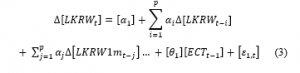
The extension of (3) of two variables into six variables shall be expressed as follow:

where △ is the difference coefficient, and ΕСТ t-1 is the term describing the long-term equilibrium relation of the estimation coefficient as an error correction term, where α β θ is the measurement coefficient value, p is the time difference and ε_t is the error term. The Granger causality test verifies the significance of the coefficient values measured in relation to the lagged variable j and the variable i. If “H_null : j does not granger cause i” is rejected, j shall become a Granger cause to i. Impulse response verification measures how quickly information is passed between variables when impacts are delivered to the VECM model with time lag. In other words, this study analyzed how the variables in the model react with time when a certain amount of impact is delivered. A variance decomposition analysis shows the relative importance of variables, as the estimation error of VECM shows the proportion that is explained by its own and other variables. Therefore, if there is no decomposition value of the variable due to the impact of the residual, this variable is considered as exogenous.

4. Analysis data

4.1. data

The analysis variables are summarized in Table 2. The analysis period is from December 1, 2014 to November 30, 2017, and is daily closing data. The closing price is determined by the accumulation of both new information for the day and trading activities between the parties. The data was obtained through Bloomberg or heads, are organizational devices that guide the reader through your paper. There are two types: component heads and text heads.

Table 2: Analysis variables

	Market	Variables
	Global	US Treasury 10 Year
		Credit spread
		VIX index
		TED spread
Korea	onshore	KRW
	offshore	KWD1m
China	onshore	CNY
	offshore	CNH*, CNK**
Japan	Global	JPY

The exchange rate is the spot exchange rate. SPOT of the Chinese yuan, the Japanese yen, and the Korean won, against U.S. dollar.  The Chinese yuan is analyzed by dividing it into onshore yuan (CNY) and offshore yuan in Hongkong (CNH).  For the Korea won dollar, there is no offshore spot exchange rate. Therefore, the shortest term of one-month term in offshore market was used as a won-dollar offshore exchange rate (KWD1m). The analysis variables for the international financial market are the 10-year U.S. treasury bond interest rate, Credit risk spread, VIX index and TED spread, which are daily closing data. During the analysis period, there were no fundamental shift in the international financial market, such as the 1998 Asian financial market crisis or the 2008 international financial market crisis. Therefore, dummy variables were not considered. The analysis of basic statistics of yen, yuan, and won dollar is summarized in Table 3. The spot exchange rate and the VIX index were calculated as the difference between today’s closing price taken on the log value and the previous day’s closing price taken on the log value. The 10-year treasury interest rate, credit risk spread and TED spread are the difference between today’s and the previous day’s closing price of data.

Table 3: Raw data statistic

	onshore market		Global market
	Korea	China	Korea	China		Japan	global market variable
Variables	KRW	CNY	KWD1m	CNH	CNK	JPY	T10Y	CREDIT	LVIX	TED
Mean	1141.52	6.55	1142.34	6.56	174.38	114.17	2.09	1.70	14.72	34.53
Median	1136.95	6.58	1137.69	6.58	174.61	113.62	2.17	1.66	13.72	31.38
Maximum	1240.90	6.96	1246.00	6.98	189.53	125.63	2.63	2.30	40.74	68.93
Minimum	1068.60	6.15	1064.95	6.15	162.01	100.03	1.36	1.29	9.14	14.52
Std. Dev.	35.29009	0.24247	34.99482	0.23624	7.00772	6.40875	0.28092	0.23559	4.25084	10.46365
Observations	784	784	784	784	784	784	784	784	784	784
ADF	-2.1636	-1.6404	-2.1636	-1.7592	-1.5864	-1.5845	-2.1857	-0.3129	-4.5982***	-2.2357
PP	-2.2105	-1.6339	-2.2105	-1.7090	-1.3730	-1.5983	-2.0749	-0.6730	-4.4872***	-2.1803

* 10% significance level, ** 5% significance level, *** 1% significance level. KRW, CNY, and JPY are Korean, Chinese and Japanese spot exchange rates. CNH is the Chinese offshore yuan spot exchange rate, and KWD1m is the 1-month NDF KRW exchange rate. T10Y is the US treasury 10-year interest rate (%). CREDIT is the difference (%) of the spread between T10y and BBB credit rating bonds. VIX is the chicago options market index (%). TED is the difference between the libor 3-month interest rate and the T-bill rate (basis point)

Table 4: Stationary test

	onshore market		Global market
	Korea	China	Korea	China		Japan	global market variable
	KRW	CNY	KWD1m	CNH	CNK	JPY	T10Y	CREDIT	LVIX	TED
ADF	-2.1636	-1.6404	-2.1636	-1.7592	-1.5864	-1.5845	-2.1857	-0.3129	-4.59***	-2.2357
PP	-2.2105	-1.6339	-2.2105	-1.7090	-1.3730	-1.5983	-2.0749	-0.6730	-4.48***	-2.1803
ADF	-27.09***	-24.50***	-28.91***	-20.61***	-25.75***	-27.44***	-30.12***	-27.41***	-27.71***	-11.79***
PP	-27.07***	-24.43***	-29.03***	-24.56***	-25.73***	-27.44***	-30.13***	-42.64***	-30.09***	-27.92***

4.2. Data

The Stationary of the data was confirmed prior to the analysis. The study used ADF (Augmented Dickey Fuller) and PP (Phillips-Perron) unit root analysis method to verify the data. The analysis result of the yen, the yuan, and the won and international financial market variables are summarized in Table 4.

The first difference of the natural logarithm of spot exchange rate and VIX index data rejected the null hypothesis that “there is a unit root”. Therefore, time series data satisfy the stationary condition. The first differenced data of 10-year US treasury interest rate (T10Y), Credit risk spread (CREDIT) and TED spread (TED) showed that the data satisfied the stationary without the unit root. Therefore, this study analyzed by using the log conversion for spot exchange rate, and VIX index data, and by using the level data for the US treasury 10-year interest rate, Credit risk spread, and TED spread.

4.3. Cointegration Test

The optimal time lag of the fifteen VECM model among the aforementioned six variables was determined prior to the cointegration test between the analytic variables. The optimal time lag was selected based on the time differences where AIC and SC values are minimized in the Akaike Information Criteria (AIC) or Schwarz Criteria (SC) analysis. The results of the time lag selection of the VECM (p) model are summarized in Table 6 below. The optimal time lag of the yen and Korea won is the time lag 3. The optimal time lag of the Chinese yuan is time lag 6. In the case of the yuan, the long-term equilibrium cointegration relationship was found to lag behind the yen and the won dollar. The time lag determined for each VECM model was applied to both the cointegration verification and the VECM analysis. The following includes the examination of whether there is at least one cointegration vector, which is a long-term equilibrium relationship between level variables of each time-series data, through cointegration analysis commonly used in financial time series data analysis. Table 5 summarizes the results of the number of the cointegration analysis of fifteen VECM analysis model between the analytic variables.

As summarized in Table 5, the null hypothesis of “no cointegration vector” was rejected at the 5% level for the all fifteen analysis model cases. Therefore, more than one cointegration relation between time series variables used in fifteen analysis model was revealed. The existence of the cointegration indicates that the individual variables are non-stationary, but when they are linked by a cointegration vector relation it indicates the stationary. Therefore, this study analyzed the lead-lag causality between variables using the VECM analysis model that includes the error correction term in the VAR model analysis.

Table 5: Cointegration vector

Currency		market sector (model No)		Cointegration vectors
						dependent	independent variable
K R W	on-shore K R W	[CNK] KWD1m, KRW, CNH, CNY, JPY	(1)		constant	LCNK	LKWD1m	LKRW	LCNH	LCNY	LJPY
				Coint EQ (1)	-4.49	1	0	0	-25.97316***	25.92838***	-0.118494
				Coint EQ (2)	-4.62	0	1	0	-26.39582***	25.37661***	-0.099479
				Coint EQ (3)	-4.55	0	0	1	-26.64894***	25.60423***	-0.104134
		[KRW] KWD1m, CNK, CNH, CNY, JPY	(2)		constant	LKRW	LKWD1m	LCNK	LCNH	LCNY	LJPY
				Coint EQ (1)	-4.55	1	0	0	-26.64894***	25.60423***	-0.104134
				Coint EQ (2)	-4.62	0	1	0	-26.39582***	25.37661***	-0.099479
				Coint EQ (3)	-4.49	0	0	1	-25.97316***	25.92838***	-0.118494
		[KRW] KWD1m	(3)		constant	LKRW	LKWD1m
				Coint EQ (1)	0.11	1	-1.015389***
		[KRW] KWD1m, T10Y, Credit, VIX, TED	(4)		constant	LKRW	LKWD1M	T10Y	CREDIT	LVIX	TED
				Coint EQ (1)	-8.52	1	0	0.081849	-0.895473***	1.074763***	-0.000894
				Coint EQ (2)	-8.47	0	1	0.079503	-0.872705***	1.044728***	-0.000904
	off-shore K W D 1m	[KWD1m] KRW, CNK, CNH, CNY, JPY	(5)		constant	LKWD1m	LKRW	LCNK	LCNH	LCNY	LJPY
				Coint EQ (1)	-4.62	1	0	0	-26.39582***	25.37661***	-0.099479
				Coint EQ (2)	-4.55	0	1	0	-26.64894***	25.60423***	-0.104134
				Coint EQ (3)	-4.49	0	0	1	-25.97316***	25.92838***	-0.118494
		[KWD1m] KRW	(6)		constant	LKWD1m	LKRW
				Coint EQ (1)	-0.11	1	-0.984844***
		[KWD1m] KRW, T10Y, Credit, VIX, TED	(7)		constant	LKWD1m	LKRW	T10Y	CREDIT	LVIX	TED
				Coint EQ (1)	-9.44	1	0	0.153340	-1.253755***	1.587332***	-0.000418
				Coint EQ (2)	-9.52	0	1	0.158203	-1.290331***	1.636855***	-0.000389
R M B	on-shore C N Y	[CNY] CNH, CNK, KWD1m, KRW, JPY	(8)		constant	LCNY	LCNH	LCNK	LKWD1m	LKRW	LJPY
				Coint EQ (1)	-7.33	1	0	0	64.16184***	-63.55239***	0.235192
				Coint EQ (2)	-6.87	0	1	0	61.64652***	-61.09849***	0.229879
				Coint EQ (3)	7.09	0	0	1	-62.4577***	60.8898***	-0.245945
		[CNY] CNH	(9)		constant	LCNY	LCNH
				Coint EQ (1)	0.06	1	-1.030136***
		[CNY} CNH, T10Y, Credit, VIX, TED	(10)		constant	LCNY	LCNH	T10Y	CREDIT	LVIX	TED
				Coint EQ (1)	-12.80	1	0	0.773481	-4.477629***	6.285092***	0.005925
				Coint EQ (2)	-12.96	0	1	0.786428	-4.551355***	6.38005***	0.006126
	off-shore C N H	[CNH] CNY, CNK	(11)		constant	LCNH	LCNY	LCNK
				Coint EQ (1)	0.23	1	-1.004402***	-0.04332***
		[CNH] CNY, CNK KWD1m, KRW, JPY	(12)		constant	LCNH	LCNY	LCNK	LKWD1M	LKRW	LJPY
				Coint EQ (1)	-6.87	1	0	0	61.64652***	-61.09849***	0.229879
				Coint EQ (2)	-7.33	0	1	0	64.16184***	-63.55239***	0.235192
				Coint EQ (3)	7.09	0	0	1	-62.4577***	60.8898***	-0.245945
		[CNH] CNY	(13)		constant	LCNH	LCNY
				Coint EQ (1)	-0.06	1	-0.969678***
		[CNH] CNY, T10Y, Credit VIX, TED	(14)		constant	LCNH	LCNY	T10Y	CREDIT	LVIX	TED
				Coint EQ (1)	-5.27	1	0	0.194119	-1.489189***	2.081043*	-0.000288
				Coint EQ (2)	-5.25	0	1	0.192055	-1.473122***	2.066396*	-0.000370
JPY	[JPY] T10Y, Credit, VIX, TED		(15)		constant	JPY		T10Y	CREDIT	LVIX	TED
				Coint EQ (1)	-2.87	1		-0.22638***	0.524198***	-0.882197***	0.002019

5. Analysis Result

5.1. VECM Analysis

Table 6 shows the relationship between the rate of change of the analytic variables by applying the time lags to the fifteen VECM model using the long-term cointegrating equilibrium equations. The fifteen VECM analysis models’ error correction term, ECT values are expressed as Coint EQ (1). In the VECM model analysis, if there are two cointegrations, it is expressed as Coint EQ (1) and (2). In the VECM analysis model, the ECT, error correction term must be negative (-) and statistically significant at the same time. Table 6 analysis results showed that 12 of the total 15 analysis models had negative (-) error correction terms and were statistically significant at the same time. However, in analysis models 5, 6 and 12, the error correction term was negative (-), but it was not significant.

* Korea won dollar and Seoul offshore yuan

We found four onshore won-dollar models, three offshore won-dollar models, and a total of seven VECM analysis models. The following Table 6 shows that all four VECM models of the onshore won-dollar were significant.  The long-term equilibrium relationship explanation power of the VECM model was found to be around 50 percent to 68 percent. However, the explanation power of the three offshore won-dollar VECM models was about 3 percent to 6 percent. The error correction term, Coint EQ of the five VECM analysis models was negative (-) and statistically significant. However, analysis models No. 5 and No. 6 showed that the error correction term were negative (-), but were not statistically significant. The VECM Model No. 1, CNK, shows a long-term equilibrium relationship between the won-dollar and the yuan and the yen. Since CNK is an offshore yuan traded in the Seoul foreign exchange market, there are no restrictions on its transactions. Therefore, it has been shown that the Seoul offshore yuan (CNK) has a long-term equilibrium relationship with onshore yuan (CNY) and offshore yuan (CNH) and Japanese yen (JPY) either. These results suggest that although the yuan’s liquidity in the Seoul foreign exchange market is relatively insufficient compared to Hong Kong. Therefore, it secures insufficient liquidity through cross-rate transactions between currencies of KRW↔USD↔CNH, CNY, and JPY. The amount of liquidity of a currency used in transactions turned out to be the influence factor of these currencies. It gives impact on the Seoul offshore yuan (CNK) exchange rate either. VECM model No. 2, onshore won-dollar (KRW) exchange rate, indicated that there was a long-term equilibrium relationship with the offshore won-dollar exchange rate, the yuan and the yen. This result implied that the won-dollar exchange rate received impact by the yuan and yen flowing through the export/import trade and inter-bank money markets transactions between Korea, China, and Japan. VECM Model No. 4 is an analysis of the relationship between the onshore won-dollar (KRW) and the variables in the international financial market. The analysis results indicated that the won-dollar exchange rate has a long-term equilibrium relationship with variables in the international financial market. VECM Analysis Models No. 1, No. 2, No. 3 and 4 show that the error correction factor of the offshore won-dollar exchange rate (KWD1m) is greater than that of the other variables. VECM model No. 3 analyzed the relationship between two variables, the onshore won-dollar exchange rate (KRW) and the offshore won-dollar (KWD1m). According to the analysis of the long-term equilibrium relationship between the two variables, the offshore won-dollar exchange rate explains the onshore won-dollar exchange rate about 50%. These results are similar to [47] the author’s argument. They studied the Granger causal relationship between the KRW exchange rate and the offshore NDF KRW market. They argued that the offshore one-month forward exchange market was strongly causative in the onshore spot exchange market and that the volatility shock was exchanged between the two markets. In [34] the author analyzed the relationship between offshore yuan (CNH) and onshore yuan (CNY) for the period from September 2010 to August 2013. They argued that the CNH Hong Kong yuan has a predictive power for the CNY yuan in China. The Korean won has not yet been internationalized, but like the yuan, the onshore won-dollar exchange rate has been consistently and strongly influenced by the offshore market won-dollar exchange rate. In addition, the offshore won-dollar exchange rate, KWD1m is found to have a long-term equilibrium relationship with four variables in the international financial market, and as a result, the Korean won-dollar exchange rate (KRW) is affected by variables in the international financial market either. The results suggest that Korea onshore won-dollar exchange market and the Korea won-

Table 6: VECM analysis

KRW

Yuan

JPY

[dependent variable]

[onshore KRW]

[offshore KWD1m]

[onshore CNY]

[off-shore CNH]

[CNK]

[KRW]

[KRW]

[KRW]

[KWD1m]

[KWD1m]

[KWD1m]

[CNY]

[CNY]

[CNY]

[CNH]

[CNH]

[CNH]

[CNH]

[JPY]

variable 1

LKWD1m

LKRW1m

LKWD1m

LKRW1m

LKRW

LKRW

LKRW

LCNH

LCNH

LCNH

LCNY

LCNY

LCNY

LCNY

variable 2

LKRW

LCNK

T10Y

LCNK

T10Y

LCNK

T10Y

LCNK

LCNK

T10Y

T10Y

variable 3

LCNH

LCNH

CREDIT

LCNH

CREDIT

LKRW1m

CREDIT

LKWD1m

CREDIT

CREDIT

variable 4

LCNY

LCNY

LVIX

LCNY

LVIX

LKRW

LVIX

LKRW

LVIX

LVIX

variable 5

LJPY

LJPY

TED

LJPY

TED

LJPY

TED

LJPY

TED

TED

Coint EQ (1)

-0.43***

-0.584***

-0.60***

-0.617***

-0.1303

-0.0646

-0.1747**

-0.056**

-0.035*

-0.058**

-0.064**

-0.0455

-0.051*

-0.063*

-0.002*

Coint EQ (2)

-0.1237

0.2444***

0.16879**

0.6307***

0.6114

0.6353***

0.1095*

0.05109

0.0261

0.065***

Coint EQ (3)

-0.0416

0.0911**

0.3452***

-0.191***

-0.235***

time lag

3

3

2

3

3

2

3

3

4

3

4

3

6

2

3

adjusted R^2

68.48%

50.94%

49.97%

51.29%

3.21%

0.66%

6.47%

7.92%

7.34%

8.63%

4.78%

5.25%

5.46%

4.93%

9.42%

model number

(1)

(2)

(3)

(4)

(5)

(6)

(7)

(8)

(9)

(10)

(11)

(12)

(13)

(14)

(15)

government bond market and the inter-bank money market are substantially and effectively open, so this increase the link to the international financial market. In [49] the author and in [50] the  announcement argued that certain currency shocks are transferred through the interbank money market. It also argued that the impact from the US dollar currency affects the interbank money markets in Hong Kong (HKD), Australia (AUD), Japan (JPY), and Korea (KRW). However, they argued that the impact of the US dollar currency impact on China (Yuan), Thailand (THB) and Malaysia (RHB) is limited. The fact that the Korean won dollar exchange rate is strongly related to the international financial market is in line with [49] the author’s argument and with [50] announcement. The VECM model relationships model No. 5 and model No. 6 were not significant. The analysis shows that offshore won-dollar exchange rates are more affected by international financial market factors than by regional factors between Korea, China and Japan in Northeast Asia.

*China Yuan

We found three onshore analysis model and four offshore analysis models, and a total of seven VECM analysis models. The three VECM models of the onshore yuan (CNY) were shown to be statistically significant. The three long-term equilibrium relationship VECM models of the onshore yuan had the explanatory power of between 7% and 8%. The explanatory power of the four VECM models of the Hong Kong offshore yuan (CNH) was between 4% and 5%. Although the error correction term of the six VECM analysis models was significant, analysis model 12 showed that the error correction term was not significant.  The VECM model No. 8 Chinese onshore yuan (CNY) was found to have a long-term equilibrium relationship with the onshore won dollar (KRW) and the yen (JPY). The analysis results of VECM Model No. 10 and No. 14 show that onshore and offshore yuan have long-term equilibrium relationship with international financial market variables. The VECM model No. 11 Hong Kong offshore yuan (CNH) has a long-term equilibrium relationship with the Chinese onshore yuan (CNY) and the Korean offshore yuan (CNK). The unusual was that, VECM analysis models No. 9 and 13, show that China’s long-term equilibrium relationship between onshore and offshore yuan is weaker than Korea’s onshore and offshore won-dollar relations. In the previous model No. 3 Korean Won-dollar VECM analysis model, offshore Won-dollar’s explanation power on the onshore KRW was about 50%, at 1% significant level. However, the explanatory power of the VECM No. 9 and No. 13 analytical models analyzed the Chinese yuan was 7.3% and 5.4%, respectively, and it was found to be significant at the 10% level. It is unusual for the long-term equilibrium relationship between onshore and offshore yuan markets to be weaker than the non-international currency of Korea won. This analysis result is interpreted by the fact that the yuan onshore-offshore trade related cross border transactions are liberalized, but capital market transactions are limited. Overall, the yuan’s long-term equilibrium relationship with other currencies was weaker than that of Korea won. And these results are in line with [49] the author’s argument that the impact of the shock from the US dollar currency on Chinese yuan is limited.

*Japan Yen

VECM Analysis Model No. 15 of Table 6 is the result of an analysis of the long-term equilibrium relationship between the Japanese yen and variables in the international financial market. The analysis indicated that the yen exchange rate is more related to the variables in the international financial market than that of the won and the yuan. This result suggest that the yen is international currency and the Japanese bond markets are fully open to international financial market investors, so, the greater association with the variables of the international financial market than the non-international currency, the Korea won and the yuan, which is on the way of internationalized. Analysis models 1, 2, and 8 show that the onshore won dollar (KRW) and the onshore yuan (CNY) have a long-term equilibrium relationship with the yen (JPY). This result show that since most of the demand and supply of foreign exchange transactions occurred through import-export transactions and were supplied to the foreign exchange markets in Korea and China, so the currency market result in long term equilibrium relationship. However, looking at analysis models Nos. 5, 6, and 12, it was found that the offshore won (KWD1m) and the offshore yuan (CNH) had no long-term equilibrium relationship with the yen (JPY). This result is interpreted as that, in the offshore international financial market, since investors trade currencies in consideration of the country risk of the currency, a long-term equilibrium relationship between the offshore won and the offshore yuan is not established with the international currency, the yen.

5.2. Granger Causality Analysis

The VECM model has no restriction on the analytical model and may cause a fictitious spurious regression analysis problem. As such, this study further conducted a widely used in time series analysis, Granger causality test. The null hypothesis of Granger causality test is that “the offshore won, KWD1m has no effect on the spot exchange rate of the onshore won, KRW”, and the direction of the causal relationship in Table 7 was written as “KWD1m→KRW”. If the null hypothesis is rejected, the offshore won shall have an impact on onshore KRW exchange rates. Table 7 summarizes the results of the Granger causality analysis between the exchange rates of Japanese yen, Chinese renminbi, and Korean won, and between the exchange rates of the three currencies of Korea, China, and Japan and variables in the international financial market.

Table 7: Granger Causality analysis of won, yuan, yen and international financial market variables

Currency		market sector (model No)		Granger Causality relation			Time lag (1)	Time lag (2)	Time lag (3)	Time lag (4)	Time lag (5)
							Chi-square	Chi-square	Chi-square	Chi-square	Chi-square
K R W	on-shore K R W	[CNK] KWD1m, KRW, CNH, CNY, JPY	(1)	KWD1m	→	CNK	14.9383	56.2589	214.79	165.636	135.221
				CNH	→	CNK	na	na	na	2.94628**	2.39355**
				CNY	→	CNK	3.33834*	na	na	2.05321*	na
				KRW	→	CNK	na	77.2157***	58.6483***	45.4459***	36.4794***
				JPY	→	CNK	6.40453**	3.18475**	3.45293**	3.06304**	2.74506**
				CNK	→	KWD1m	na	na	na	na	na
				KRW	→	KWD1m	na	na	na	na	na
				CNH	→	KWD1m	na	na	na	na	na
				CNY	→	KWD1m	na	na	na	na	na
				JPY	→	KWD1m	na	na	na	na	na
				KWD1m	→	KRW	732.949***	379.449***	254.111***	189.808***	152.381***
				CNK	→	KRW	na		2.49953*	2.63884**	2.13671*
				CNH	→	KRW	na	16.3348***	13.3646***	10.049***	9.04209***
				CNY	→	KRW	na	12.1681***	10.988***	8.23484***	6.57248***
				JPY	→	KRW	na	5.78389***	6.56095***	5.00083***	4.69926***
				CNY	→	CNH	4.22086**	6.22332***	3.6091**	2.61292**	2.23464**
				CNK	→	CNH	na	na	na	na	na
				LKWD1m	→	CNH	na	na	na	na	na
				KRW	→	CNH	na	na	na	na	na
				JPY	→	CNH	na	na	na	na	na
				CNK	→	CNY	na	na	na	na	na
				LKWD1m	→	CNY	na	na	na	na	na
				KRW	→	CNY	na	na	na	na	na
				CNH	→	CNY	13.5758***	14.8769***	11.4008**	8.35465***	6.67746***
				JPY	→	CNY	na	na	na	na	na
				KWD1m	→	JPY	2.99698*	na	na	na	na
				KRW	→	JPY	3.07157***	na	na	2.07901*	2.3439**
				CNK	→	JPY	na	na	na	na	na
				CNH	→	JPY	na	na	na	na	na
				CNY	→	JPY	na	na	na	na	na
			(2)	[KRW] KWD1m, CNK, CNH, CNY, JPY
			(3)	[KRW] KWD1m
		[KRW] KWD1m, T10Y, Credit, VIX, TED	(4)	T10Y	→	KRW	na	na	4.50778***	3.50753***	3.53952***
				Credit	→	KRW	3.33958**	na	na	na	na
				VIX	→	KRW	5.16845**	4.82868***	5.68474***	4.39125***	3.57154***
				T10Y	→	KWD1m	na	2.86013*	2.92025**	3.17319**	3.53952***
				Credit	→	KWD1m	4.01793**	na	na	na	na
				TED	→	KWD1m	na	4.19474**	2.73643**	3.00317**	2.4705**
				KWD1m	→	T10Y	na	3.16114**	2.02383*	2.48292**	1.8993*
	off-shore KWD1m		(5)	[KWD1m] KRW, CNK, CNH, CNY, JPY
			(6)	[KWD1m] KRW
			(7)	[KWD1M] KRW, T10Y, Credit, VIX, TED
R M B	on-shore C N Y		(8)	[CNY] CNH, CNK, KWD1m, KRW, JPY
			(9)	[CNY] CNH
		[CNY] CNH, T10Y, Credit, VIX, TED	(10)	TED	→	CNY	3.57194**	3.87336**	2.81656**	2.17497*	1.95067*
				CNY	→	Credit	3.76118*	2.47433*	na	na	na
				CNY	→	VIX	5.01105**	3.03027**	na	na	na
				CNY	→	TED	na	na	na	na	1.86105*
	off-shore C N H		(11)	[CNH] CNY, CNK,
			(12)	[CNH] CNY, CNK, KWD1m, KRW, JPY
			(13)	[CNH] CNY
		[CNH] CNY, T10Y, Credit VIX, TED	(14)	TED	→	CNH	na	3.64619**	2.49048*	na	na
				CNH	→	Credit	3.52004*	3.13441**	3.03439**	2.40199**	2.44063**
				CNH	→	VIX	3.4716*	2.36669*	na	na	na
J P Y	[JPY] T10Y, Credit, VIX, TED		(15)	T10Y	→	JPY	na	6.90707***	5.24848**	4.46118***	3.72127***
				Credit	→	JPY	na	14.591***	13.7139***	10.8005***	8.83545***
				VIX	→	JPY	na	3.52556**	2.28807*	na	na
				TED	→	JPY	3.00953*	6.51429***	4.74023***	4.46049***	4.40631***
				JPY	→	T10Y	na	na	na	na	na
				JPY	→	Credit	7.08832***	10.0327***	6.64887***	4.78381***	4.11865***
				JPY	→	VIX	6.24512**	4.23995**	2.92458**	2.29145*	1.9398*
				JPY	→	TED	na	3.43594**	2.43067*	na	2.01376*

* (KWD1m → KRW) the direction of the arrow is the direction of the granger causal relationship. ‘na’ is no the granger causal relationship does not exist at the significance level. The Granger causal relationship analysis results of  analysis models 2, 3, 5 to 9, 11 to 13 are overlapped with model 1

*Korea won dollar and Seoul offshore yuan

Models No. 1 through No. 4 in Table 7 summarizes the variables affecting the Granger causal relationship between the Korean won (KRW) and the Seoul offshore yuan (CNH). The causality analysis among the variables showed that offshore won (KWD1m) was the biggest cause-and-effectiveness for Korean onshore won (KRW). After KWD1m, the onshore won exchange rate was shown to be causal in the order of Hong Kong’s offshore yuan (CNH), China’s onshore yuan (CNY) and Japan’s yen (JPY) at 1% significant level. These results suggest that the offshore won-dollar exchange rate had the greatest impact on the onshore won-dollar exchange rate. And it is in line with the findings of [34] the author who claimed that the influence of the Chinese offshore yuan on the onshore yuan has increased. The unusual was that the Chinese yuan causes more on the onshore won dollar exchange rate than the yen. These results are interpreted as reflecting the largest export-import trade volume of Korea with China. Model 4 analyzed the Granger causal relationship between the won dollar and international financial market variables. The analysis results show that 10-year US treasury bonds, Credit risk spread, and VIX index causes Korean onshore won dollars (KRW) at 1%, 5%, and 1% significance levels, respectively. Models No. 5 through 7 analyzed and summarized the variables affecting causality in offshore won dollars. According to the Granger causal analysis among the variables, the offshore won-dollar exchange rate (KWD1m) has no causal relationship with the onshore dollar, the Hong Kong Overseas Yuan (CNH), the Chinese onshore yuan (CNY) and yen (JPY). Similar to this analysis, the analysis results of VECM model No. 5 showed that offshore won has no long-term equilibrium with the yuan and yen. In [51] the author argued that the depreciation of the exchange rate is an increase in the sovereign credit risk. The analysis results of this paper and in [51] the author reconfirm that when international financial market investors trade offshore won (KWD1m), they trade based on the expected rate of return versus risk considering the country-specific factor only. In addition, offshore dollars are freely traded in overseas markets without being restricted by Korea foreign exchange transaction regulations, and the difference in price at maturity is settled in US dollars. Therefore, the absence of a liquidity problem in offshore won have affected the analysis results. This analysis result is reconfirmed in the Granger causality relationship analysis result of the model 7 variables. International financial market variables such as US 10-year treasury bonds, Credit risk spread, and TED spread were found to cause offshore won dollars (KWD1m) at 1%, 5%, and 5% significant level, respectively. The results of the Granger causality relationship analysis of Models 5 and 7 show that the offshore won-dollar exchange rate has no causal relationship with the yuan and yen but has a causal relationship with international financial market variables. These results provide policy implications that the analysis of future won-dollar exchange rate fluctuations should be approached from the perspective of global investment portfolio investor in international market.

*China Yuan

Models 8 to 10 in Table 7 summarize variables that have a Granger causal effect on the Chinese onshore yuan (CNY). Since the variables used in the Granger causal relationship analysis are the same as those of models 1 to 4, we need to refer the analysis result of model 1. The analysis results of this study showed that the Hong Kong offshore yuan, CNH was causal to the Chinese onshore yuan (CNY) at a significance level of 1%.  However, it was found that the Seoul offshore yuan (CNK), the offshore won dollar (KWD1m), the onshore won dollar (KRW), and the Japanese yen (JPY) do not cause the Chinese onshore yuan (CNY). Model No. 10, the analysis of Granger causality between the yuan and the variables in the international financial market showed that only the TED spread Granger causal the yuan at a 5% significance level. However, 10-year US treasury interest rate, the Credit risk spread, the VIX index did not cause onshore yuan. Models 11-14 summarize the variables that have a Granger causal effect on the Hong Kong offshore yuan (CNH). Since the variables used in the Granger causal relationship analysis are the same as those of models 1 to 4, we refer to the ones summarized in model 1. According to the results of Granger causal relationship analysis between variables, it was found that the Chinese onshore yuan (CNY) caused the Hong Kong offshore yuan (CNH) at a 1% significance level. In the model 14, the analysis of the Granger causal relationship between the offshore yuan and the variables of the international financial market variables, it was found that only TED spread caused Hong Kong offshore yuan (CNH) at a 5% significance level. However, similar to the onshore yuan (CNY), the 10-year US treasury interest rate, Credit risk spread, VIX index, did not appear to be Granger causal to the Hong Kong offshore yuan (CNH). These results show that since dollar liquidity required for currency exchange transactions is secured through the interbank money market, the TED spread, which represents the level of liquidity in the interbank money market, has an impact. In the case of Korean won, the offshore won dollar market caused onshore won, but not in the opposite case. In the case of the yuan, however, it was found that the onshore-offshore yuan exchanged its causal relationship. In [35] the author argued that yuan liquidity and risk aversion of investors in international financial markets are the main reasons for creating price differences and generating profit-taking arbitrage transaction between CNY and CNH. They argued that increased inflow of yuan from the onshore CNY market to the Hong Kong CNH offshore market would reduce the difference in CNH-CNY prices, so that the yuan exchange rate would be adjusted based on the onshore CNY, which has more liquidity. According to [50] the statement, China began supplying yuan liquidity to Hong Kong’s offshore markets in cooperation with HKMA on November 10, 2014. Therefore, the onshore yuan’s Granger causal of offshore yuan is showed. Offshore yuan have been influenced by the ample liquidity of the onshore yuan market. In [34] the author analyzed CNH and CNY markets for the period from September 2010 to August 2013. They argued that CNH’s influence on CNY has increased, and argued that CNH Hong Kong offshore yuan has predictive power over CNY China onshore yuan. The onshore yuan market is limited to investors in the international financial market, while the Hong Kong currency market has no trading limitation. Therefore, as argued by [34] the author, it has been shown that the price-discovery effect of the Hong Kong offshore yuan market may have affected the onshore yuan market. The yuan (CNY and CNH), the SDR currency, is the same yuan, but the onshore yuan and the offshore yuan exchange each other’s independent causal relationship and each has a distinct characteristic. These analysis results provide important implications for investment and risk-hedge transactions for companies that use the yuan to trade in import-exports and for investors in the international financial market.

*Japan Yen

Model 15 of Table 7 summarizes the Granger causal relationship of international financial market variables to the Japanese yen. The analysis results showed that all four variables (the 10-year US treasury bond, credit risk spread, VIX index, and TED spread) were responsible for the change in the yen’s exchange rate at 1%, 1%, 5%, and 1%, significant level respectively. The aforementioned analysis of the Korean won dollar showed that three variables in the international financial market affect the won-dollar exchange rate. In yuan case, only TED spread affects the yuan’s exchange rate. It was expected that the yen, the international currency, would be the strongest in the strength of Granger causality relationship among the variables in the international financial market, Chinese the yuan that is in the process of internationalization, would be the next and the won-dollar, the non-international currency would be the weakest. However, the analysis result showed that the non-international currency, the won, has a stronger Granger causal relationship with variables in the international financial market than that of Chinese the yuan. In [14] the author analyzed the effects of international financial market variables and currency exchange rates on the country CDS premium. They argued that the Granger causal relationship of the international financial market variables and the won-dollar exchange rate that affect the Korea country CDS premium is stronger than that of the China country CDS premium. Therefore, when a shock occurs in the international financial market, the shock could be dispersed and absorbed into the Korea CDS premium and the onshore and offshore won-dollar currency market. However, for China the shock could be concentrated in the CDS premium only. The analysis results that the Korean won dollar has a stronger Granger causal relationship with international financial market variables than the Chinese yuan is in line with their arguments.

5.3. Impulse Response Analysis

The Granger causality test informs the direction of the causal relationship between variables. However, the Granger causality test cannot determine whether the direction of the causal relationship is positive (+) or negative (-). Therefore, the impulse response analysis was performed to measure the impact of a specific variable on other variables. The Impulse response results are summarized in Table 8 for the results of the 1 to 10th and 20th, and 30th days.

Table 8: Impulse response analysis of won, yuan, yen and international financial market variables

Curr -ency		model number		Response of dependents variable to one standard deviation of innovations								Currency		model number		Response of dependents variable to one standard deviation of innovations
				days	depen -dent	independent variables										days	depen -dent	independent variables
K R W	on-shore K R W	[CNK] KWD 1m, KRW CNH CNY JPY	(1)		LCNK	LKRW1m	LKRW	LCNH	LCNY	LJPY		R M B	on-shore C N Y	[CNY] CNH CNK KWD 1m, KRW JPY	(8)		LCNY	LCNH	LCNK	LKRW1M	LKRW	LJPY
				1 day	0.00261	0.00000	0.00000	0.00000	0.00000	0.00000						1 day	0.00182	0.00000	0.00000	0.00000	0.00000	0.00000
				2 day	0.00110	0.00163	0.00062	(0.00087)	(0.00004)	(0.00002)						2 day	0.00210	0.00038	(0.00006)	(0.00005)	0.00000	(0.00004)
				3 day	0.00074	0.00412	0.00031	(0.00175)	(0.00052)	(0.00010)						3 day	0.00195	0.00044	(0.00003)	(0.00008)	0.00007	(0.00003)
				4 day	0.00034	0.00399	0.00024	(0.00207)	(0.00077)	0.00039						4 day	0.00206	0.00041	(0.00006)	(0.00011)	0.00014	(0.00004)
				5 day	0.00020	0.00400	0.00022	(0.00196)	(0.00055)	0.00062						5 day	0.00209	0.00043	(0.00004)	(0.00009)	0.00011	(0.00005)
				6 day	0.00002	0.00399	0.00054	(0.00184)	(0.00067)	0.00072						6 day	0.00206	0.00045	(0.00004)	(0.00009)	0.00008	(0.00005)
				7 day	(0.00005)	0.00394	0.00081	(0.00176)	(0.00094)	0.00073						7 day	0.00208	0.00046	(0.00004)	(0.00009)	0.00008	(0.00005)
				8 day	(0.00011)	0.00399	0.00087	(0.00161)	(0.00107)	0.00071						8 day	0.00209	0.00048	(0.00004)	(0.00008)	0.00008	(0.00005)
				9 day	(0.00015)	0.00408	0.00084	(0.00147)	(0.00117)	0.00068						9 day	0.00209	0.00049	(0.00004)	(0.00008)	0.00007	(0.00005)
				10 day	(0.00017)	0.00414	0.00080	(0.00138)	(0.00127)	0.00067						10 day	0.00209	0.00050	(0.00003)	(0.00009)	0.00007	(0.00005)
				20 day	0.00014	0.00434	0.00060	(0.00061)	(0.00182)	0.00056						20 day	0.00211	0.00056	(0.00001)	(0.00011)	0.00006	(0.00006)
				30 day	0.00033	0.00437	0.00051	(0.00032)	(0.00201)	0.00049						30 day	0.00212	0.00058	0.00001	(0.00011)	0.00005	(0.00007)
		[KRW] KWD 1m, CNK CNH CNY JPY	(2)		LKRW	LKRW1m	LCNK	LCNH	LCNY	LJPY				[CNY] CNH	(9)		LCNY	LCNH
				1 day	0.00372	0.00000	0.00000	0.00000	0.00000	0.00000						1 day	0.00182	0.00000
				2 day	0.00236	0.00292	0.00006	0.00003	(0.00014)	(0.00007)						2 day	0.00209	0.00038
				3 day	0.00201	0.00468	0.00009	(0.00001)	(0.00003)	0.00009						3 day	0.00194	0.00044
				4 day	0.00195	0.00471	(0.00031)	(0.00010)	(0.00001)	0.00027						4 day	0.00205	0.00041
				5 day	0.00213	0.00479	(0.00022)	(0.00013)	(0.00004)	0.00053						5 day	0.00209	0.00044
				6 day	0.00227	0.00455	(0.00029)	0.00004	(0.00014)	0.00064						6 day	0.00208	0.00045
				7 day	0.00240	0.00453	(0.00032)	0.00022	(0.00027)	0.00059						7 day	0.00208	0.00046
				8 day	0.00245	0.00457	(0.00036)	0.00035	(0.00042)	0.00055						8 day	0.00209	0.00048
				9 day	0.00244	0.00461	(0.00034)	0.00047	(0.00052)	0.00052						9 day	0.00210	0.00050
				10 day	0.00241	0.00466	(0.00031)	0.00057	(0.00059)	0.00050						10 day	0.00210	0.00051
				20 day	0.00236	0.00481	0.00007	0.00125	(0.00106)	0.00038						20 day	0.00212	0.00061
				30 day	0.00233	0.00484	0.00025	0.00149	(0.00121)	0.00032						30 day	0.00213	0.00065
		[KRW] KWD 1m	(3)		LKRW	LKRW1m								[CNY] CNH T10Y Credit VIX TED	(10)		LCNY	LCNH	T10Y	CREDIT	LVIX	TED
				1 day	0.00372	0.00000										1 day	0.00182	0.00000	0.00000	0.00000	0.00000	0.00000
				2 day	0.00235	0.00292										2 day	0.00208	0.00038	0.00009	(0.00005)	0.00005	(0.00011)
				3 day	0.00203	0.00474										3 day	0.00193	0.00045	0.00012	0.00001	(0.00001)	(0.00017)
				4 day	0.00197	0.00485										4 day	0.00204	0.00043	0.00010	0.00000	(0.00001)	(0.00019)
				5 day	0.00194	0.00482										5 day	0.00206	0.00047	0.00011	0.00000	(0.00001)	(0.00015)
				6 day	0.00194	0.00481										6 day	0.00203	0.00051	0.00013	0.00000	(0.00003)	(0.00014)
				7 day	0.00195	0.00481										7 day	0.00205	0.00054	0.00013	0.00000	(0.00006)	(0.00014)
				8 day	0.00194	0.00481										8 day	0.00206	0.00057	0.00013	0.00000	(0.00007)	(0.00014)
				9 day	0.00194	0.00482										9 day	0.00206	0.00060	0.00014	0.00000	(0.00009)	(0.00014)
				10 day	0.00194	0.00482										10 day	0.00207	0.00062	0.00014	0.00000	(0.00010)	(0.00013)
				20 day	0.00194	0.00482										20 day	0.00210	0.00073	0.00017	(0.00000)	(0.00020)	(0.00012)
				30 day	0.00194	0.00482										30 day	0.00210	0.00075	0.00017	(0.00001)	(0.00023)	(0.00011)
		[KRW] KWD1m T10Y Credit VIX TED	(4)		LKRW	LKRW1m	T10Y	CREDIT	LVIX	TED			off-shore C N H	[CNH] CNY CNK	(11)		LCNH	LCNY	LCNK
				1 day	0.00371	0.00000	0.00000	0.00000	0.00000	0.00000						1 day	0.00261	0.00000	0.00000
				2 day	0.00233	0.00284	(0.00000)	0.00003	(0.00004)	(0.00030)						2 day	0.00293	0.00025	(0.00008)
				3 day	0.00201	0.00461	0.00055	0.00036	0.00037	(0.00049)						3 day	0.00269	0.00032	(0.00014)
				4 day	0.00192	0.00460	0.00073	0.00052	0.00047	(0.00040)						4 day	0.00248	0.00040	(0.00004)
				5 day	0.00203	0.00460	0.00112	0.00070	0.00038	(0.00071)						5 day	0.00244	0.00049	(0.00016)
				6 day	0.00215	0.00446	0.00136	0.00063	0.00037	(0.00090)						6 day	0.00247	0.00049	(0.00017)
				7 day	0.00216	0.00431	0.00137	0.00055	0.00032	(0.00093)						7 day	0.00245	0.00050	(0.00016)
				8 day	0.00217	0.00428	0.00138	0.00054	0.00024	(0.00089)						8 day	0.00243	0.00055	(0.00013)
				9 day	0.00217	0.00423	0.00137	0.00053	0.00016	(0.00086)						9 day	0.00240	0.00056	(0.00011)
				10 day	0.00216	0.00418	0.00136	0.00052	0.00008	(0.00084)						10 day	0.00237	0.00059	(0.00011)
				20 day	0.00212	0.00411	0.00142	0.00048	(0.00026)	(0.00083)						20 day	0.00219	0.00074	(0.00004)
				30 day	0.00211	0.00409	0.00144	0.00046	(0.00036)	(0.00083)						30 day	0.00213	0.00079	(0.00001)
	off-shore KWD1m		(5)	na	LKWD1m	LKRW	LCNK	LCNH	LCNY	LJPY					(12)	na	LCNH	LCNY	LCNK	LKRW1M	LKRW	LJPY
			(6)	na	LKWD1m	LKRW								[CNH] CNY	(13)		LCNH	LCNY
		[KWD1m] KRW T10Y Credit VIX TED	(7)		LKWD1m	LKRW	T10Y	CREDIT	LVIX	TED						1 day	0.00260	0.00000
				1 day	0.00584	0.00000	0.00000	0.00000	0.00000	0.00000						2 day	0.00291	0.00028
				2 day	0.00546	0.00003	0.00062	0.00037	0.00048	(0.00062)						3 day	0.00266	0.00035
				3 day	0.00509	0.00017	0.00101	0.00081	0.00056	(0.00062)						4 day	0.00245	0.00046
				4 day	0.00505	0.00047	0.00134	0.00082	0.00057	(0.00092)						5 day	0.00242	0.00059
				5 day	0.00473	0.00061	0.00141	0.00056	0.00054	(0.00091)						6 day	0.00235	0.00080
				6 day	0.00462	0.00067	0.00134	0.00058	0.00044	(0.00085)						7 day	0.00235	0.00069
				7 day	0.00460	0.00067	0.00131	0.00056	0.00033	(0.00079)						8 day	0.00237	0.00062
				8 day	0.00454	0.00067	0.00128	0.00055	0.00023	(0.00076)						9 day	0.00241	0.00064
				9 day	0.00452	0.00067	0.00129	0.00054	0.00016	(0.00074)						10 day	0.00240	0.00064
10 day				0.00451	0.00067	0.00130	0.00054	0.00009	(0.00075)		20 day	0.00231				0.00070
20 day				0.00445	0.00065	0.00137	0.00050	(0.00024)	(0.00075)		30 day	0.00227				0.00072
30 day				0.00442	0.00065	0.00140	0.00049	(0.00034)	(0.00075)		[CNH] CNY T10Y Credit VIX TED	(14)			LCNH	LCNY	T10Y	CREDIT	LVIX	TED
J P Y	[JPY] T10Y Credit VIX TED		(15)		JPY		T10Y	CREDIT	LVIX	TED					1 day	0.00260	0.00000	0.00000	0.00000	0.00000	0.00000
				1 day	0.00597		0.00000	0.00000	0.00000	0.00000					2 day	0.00293	0.00026	0.00002	(0.00001)	0.00006	(0.00019)
				2 day	0.00593		0.00087	(0.00131)	(0.00036)	(0.00071)					3 day	0.00268	0.00028	0.00004	0.00012	0.00003	(0.00025)
				3 day	0.00583		0.00115	(0.00156)	(0.00027)	(0.00098)					4 day	0.00255	0.00027	0.00007	0.00009	(0.00003)	(0.00025)
				4 day	0.00589		0.00137	(0.00139)	(0.00011)	(0.00136)					5 day	0.00251	0.00033	0.00008	0.00007	(0.00007)	(0.00024)
				5 day	0.00580		0.00124	(0.00143)	(0.00003)	(0.00134)					6 day	0.00248	0.00037	0.00008	0.00008	(0.00010)	(0.00024)
				6 day	0.00578		0.00121	(0.00144)	0.00009	(0.00130)					7 day	0.00244	0.00040	0.00008	0.00008	(0.00012)	(0.00024)
				7 day	0.00575		0.00124	(0.00141)	0.00021	(0.00127)					8 day	0.00240	0.00044	0.00009	0.00008	(0.00014)	(0.00024)
				8 day	0.00571		0.00122	(0.00140)	0.00032	(0.00128)					9 day	0.00236	0.00047	0.00009	0.00008	(0.00016)	(0.00024)
				9 day	0.00568		0.00122	(0.00138)	0.00042	(0.00129)					10 day	0.00233	0.00049	0.00009	0.00008	(0.00017)	(0.00025)
				10 day	0.00566		0.00122	(0.00136)	0.00050	(0.00130)					20 day	0.00211	0.00067	0.00010	0.00008	(0.00021)	(0.00026)
				20 day	0.00552		0.00121	(0.00129)	0.00093	(0.00131)					30 day	0.00203	0.00072	0.00010	0.00008	(0.00020)	(0.00026)
				30 day	0.00549		0.00121	(0.00127)	0.00104	(0.00131)

* a negative number in parentheses

*Korea won dollar and Seoul offshore yuan

Table 8 summarizes the impulse response results of 15 analysis models. The analysis results of this study showed that Model No. 1, the Seoul offshore yuan (CNK) reacts positively to the shock from the offshore dollar. It responds positively to shocks from the onshore dollar and yen. However, it reacts negatively to the shock of the yuan offshore and onshore in China. It was found that the Seoul offshore yuan currency (CNK) is most strongly affected by the impulse shock from the offshore won-dollars (KWD1m). It was found that the influence of the offshore won dollar on the Seoul offshore yuan (CNK) was greater than that of the CNH, and CNY. These results are found to be due to the fact that the lack of yuan liquidity in the Seoul offshore yuan market compared to the Hong Kong and Chinese yuan markets. It was found that the Seoul offshore yuan (CNK) market financed insufficient yuan liquidity through offshore won dollar cross rate arbitrage transaction. In addition, the impact from onshore won (KRW) and offshore won (KWD1m), Chinese onshore yuan (CNY), Hong Kong offshore yuan (CNH), and yen (JPY) to the Seoul offshore yuan (CNK) was mostly reflected within 1 to 6 time lag. This result is interpreted as the Seoul offshore yuan (CNK) exchange rate being adjusted over time through arbitrage trading between the foreign exchange markets. Model No. 2 onshore won dollar (KRW) was found to react positively to the shock from offshore won dollars. It reacts positively to shocks from the Hong Kong offshore yuan and yen. However, it reacts negatively from the shock of the Chinese onshore yuan (CNY). The onshore won dollar (KRW) has a positive response to the shock from the offshore won dollar (KWD1m) and the yen and remains constant. The onshore won dollar showed adjustment response to the impact of the offshore yuan, but a constant negative (-) response to the impact from the onshore yuan. The result is interpreted as the fact that it takes time for the onshore yuan to be delivered to the Seoul offshore yuan market through import-export transactions and limited capital market transactions. This can also be seen in the VECM analysis model No. 9 and No. 13 in Table 6 which has optimal analysis time lag was 4 and 6 days. It is also unusual for the onshore won-dollar, KRW to have different impulse reactions of the onshore yuan and offshore yuan. The onshore won-dollar showed an adjustment reaction that reverse the positive sign to negative to the impact from the Hong Kong offshore yuan (CNH). These results are interpreted that since onshore won-dollar markets and Hong Kong offshore yuan markets have no restrictions on foreign exchange trading in general, so the two markets adjust to the external shocks with cross rate arbitrage transactions. However, onshore won-dollar continuously responded negatively to the shock from the Chinese onshore yuan. The reason for such results can be interpreted that because foreign exchange transactions between the Seoul and China are only export-import related transactions are liberalized but capital market transactions are still limited, so the adjustment responses to the shocks from the outside are different. In [49] the author argued that the impact of the shock from the US dollar currency on Chinese yuan was limited. The onshore won-dollar’s negative reaction to the shock of the onshore yuan is in the same line as his argument. However, the direction of onshore and offshore yuan shock transfer to the onshore Korean won is partly opposite. This is interesting in that the impact of the yuan on the onshore won-dollar exchange rate is partially offset by offshore yuan. And these results can be interpreted that the different characteristics of the onshore and the offshore yuan contributed in part to the stabilization of the onshore won-dollar exchange rate. Models 4 and 7 onshore and offshore won dollars responded almost identically to shocks from international financial market variables. The onshore and offshore won dollar responded positively to the impact of the 10-year US treasury bond and credit risk spread. In the VIX index shock, it reacted to positive (+) and then converted to negative (-), and the shock disappeared. It responded continuously negative to the impact from the TED spread. Overall, the Korean onshore and offshore won dollar and the Japanese yen had similar shock reactions to the impact from the international financial market. However, the onshore and offshore yuan showed relatively weaker responses to shocks from variables in the international financial market than that of the won and yen. In [39] the research report argues that the determinants of investment capital inflow to emerging countries are largely influenced by factors on the supplier side, such as the level of US treasury bond rates and preference for safe assets in the international financial market. They argued that a 50bp fall in the 10-year US treasury bond yield would increase the total capital inflow to emerging countries by 13%. Korean onshore and offshore won dollars and Chinese onshore and offshore yuan responded positively to the shock arising from 10-year US treasury bonds. Rising risk free interest rates on 10-year U.S. treasury bonds increase demand for the U.S. dollar and lead to capital outflows from emerging markets, which in turn could weaken emerging economies’ currencies. This study also confirmed the results consistent with the IMF research. In [39] the research report argued that the VIX index represents the preference for safe assets in international financial markets, and that if the VIX index falls in half, the total capital inflow of emerging countries increases by 11%. However, the onshore and offshore won dollars were slightly different from the IMF argument. The impact from the VIX index was weaker than US 10-year treasury and credit spread. The reason for such results can be interpreted that, because the impact from the VIX index can be adjusted through the NDF KWD1m transaction and the offshore won dollar (KWD1m) readjusts the onshore won dollar (KRW). This result is also explained as the volume of offshore won-dollar, NDF transactions in the international financial market accounts for about 20% of the total global NDF transactions. The won dollar, the yuan, and the yen all reacted in the same negative direction to the shock from the TED spread. Changes in the TED spread implies changes in the overall liquidity level in the international financial market, or changes in credit risk levels and bond yields. In [45] the author used the TED spread as a measure of hedge funds’ liquidity level. In [49] the author argued that the impact of a particular currency is spill over through the interbank money market. As he claimed, this study also reconfirmed that the shock generated by TED spread, a variable in the international financial market, was similarly transmitted to Korea won, China yuan and Japan yen. The reason for such results can be interpreted that because banks in Korea, Japan, and China, which are counterparties in money market transactions, do not have a large difference in financing capacity in the international interbank market, and therefore all respond similarly to the shock from the TED Spread change.

*China Yuan

Table 8 summarizes the analysis results of Model No. 8, Chinese onshore yuan (CNY). CNY was found to react negatively to shocks from offshore won dollars (KWD1m), Seoul offshore yuan (CNK) and yen (JPY). On the other hand, Chinese onshore yuan responded positively to shocks from Hong Kong offshore yuan and onshore won dollar. The Chinese onshore and offshore yuan reacts positive (+) to the shocks generated from each other because the two markets are closely interconnected.  The Chinese onshore yuan (CNY) reacted positively to the shock from the Korean onshore won (KRW). This phenomenon is attributed to the fact that the 250 billion dollars import-export transactions volume between South Korea and China. Analysis of models 10 and 14, onshore and offshore yuan, and international financial market variables, showed that the onshore and offshore yuan responded similarly to shocks from international financial market variables. The unusual was that the yuan is the SDR international currency, but the response to the impact from international financial market variables was relatively weak compared to the non-international currencies Korean won and international currency Japanese yen. This phenomenon once again support [49] the author’s argument that the impact of the US dollar currency on Chinese yuan is limited.

*Japan Yen

The analysis result of model No. 15, yen, JPY summarized in Table 8 shows that JPY consistently responds to the shocks from international financial markets. The yen responded positively to shocks from 10-year US treasury bonds and credit risk spreads, and negatively (-) to shocks from the VIX index and TED spreads.

5.4. Variance Decomposition Analysis

Variance decomposition analysis is to measure the variance of the prediction error of the VECM analysis model and divide the weight for each variable. Table 9 summarized analysis result.

Table 9: Variance decomposition analysis of won, yuan, yen and international financial market variables

Curr-ency		model number		Variance decompositions of dependent variables									Curr-ency		model number		Variance decompositions of dependent variables
				days	S. E	depen -dent	independent variables										days	S. E	depen -dent	independent variables
K R W	on-shore K R W	[CNK]	(1)		S. E	LCNK	LKRW1m	LKRW	LCNH	LCNY	LJPY		R M B	on-shore C N Y	[CNY]	(8)		S. E	LCNY	LCNH	LCNK	LKRW1m	LKRW	LJPY
				10 day	0.0134	4.8881	73.8031	2.0152	13.946	3.6724	1.6745						10 day	0.0066	95.4783	4.1412	0.0407	0.1492	0.1486	0.0420
				20 day	0.0202	2.1805	77.7151	2.0285	8.3040	8.1100	1.6619						20 day	0.0095	94.4583	5.1621	0.0231	0.1807	0.1165	0.0592
				30 day	0.0254	1.4867	78.7531	1.7485	5.5444	11.006	1.4613						30 day	0.0118	93.8791	5.7306	0.0152	0.2071	0.0970	0.0711
		[KRW]	(2)		S. E	LKRW	LKWD1m	LCNK	LCNH	LCNY	LJPY				[CNY]	(9)		S. E	LCNY	LCNH
				10 day	0.0157	24.6279	73.6158	0.2814	0.3046	0.3747	0.7956						10 day	0.0066	95.7357	4.2643
				20 day	0.0234	21.2813	74.2448	0.1611	1.9899	1.6258	0.6969						20 day	0.0096	94.4312	5.5688
				30 day	0.0295	19.7039	73.5180	0.1423	3.5161	2.5471	0.5725						30 day	0.0119	93.5308	6.4692
		[KRW]	(3)		S. E	LKRW	LKWD1m								[CNY]	(10)		S. E	LCNY	LCNH	T10Y	CREDIT	LVIX	TED
				10 day	0.0156	20.5450	79.4550										10 day	0.0066	93.7528	5.4277	0.3049	0.0065	0.0673	0.4408
				20 day	0.0227	17.1122	82.8878										20 day	0.0096	91.2001	7.7013	0.4060	0.0032	0.3224	0.3671
				30 day	0.0280	16.0438	83.9562										30 day	0.0120	89.8291	8.8248	0.4644	0.0023	0.5514	0.3279
		[KRW]	(4)		S. E	LKRW	LKRW1m	T10Y	CREDIT	LVIX	TED			off-shore C N H	[CNH]	(11)		S. E	LCNH	LCNY	LCNK
				10 day	0.0154	22.8658	68.8931	4.8228	1.0169	0.3475	2.0539						10 day	0.0081	96.7287	3.0479	0.2234
				20 day	0.0220	20.6905	69.2345	6.4061	0.9974	0.2285	2.4430						20 day	0.0110	94.3654	5.4780	0.1566
				30 day	0.0270	19.9320	69.1256	7.0975	0.9654	0.2990	2.5806						30 day	0.0132	92.6297	7.2585	0.1118
	off-shore		(5)			LKWD1m	LKRW	LCNK	LCNH	LCNY	LJPY					(12)			LCNH	LCNY	LCNK	LKRW1M	LKRW	LJPY
			(6)			LKWD1m	LKRW								[CNH]	(13)		S. E	LCNH	LCNY
		[KWD1m]	(7)		S. E	LKWD1m	LKRW	T10Y	CREDIT	LVIX	TED						10 day	0.0081	95.2963	4.7037
				10 day	0.0164	89.9893	1.0681	5.0957	1.2291	0.5770	2.0409						20 day	0.0112	93.8654	6.1346
				20 day	0.0223	88.4382	1.4175	6.3739	1.1847	0.3566	2.2291						30 day	0.0135	93.0042	6.9958
				30 day	0.0270	87.6089	1.5451	7.0189	1.1424	0.3758	2.3090				[CNH]	(14)		S. E	LCNH	LCNY	T10Y	CREDIT	LVIX	TED
J P Y	[JPY] T10Y Credit VIX TED		(15)		S. E	JPY		T10Y	CREDIT	LVIX	TED						10 day	0.0081	96.9695	1.9251	0.0760	0.0863	0.1644	0.7787
				10 day	0.0195	88.1914		3.4020	4.6873	0.2073	3.5121						20 day	0.0109	94.2397	4.1311	0.1265	0.0981	0.4395	0.9650
				20 day	0.0273	86.5664		3.7050	4.7074	0.9522	4.0690						30 day	0.0129	92.2013	5.8894	0.1510	0.1067	0.5628	1.0888
				30 day	0.0333	85.6938		3.8121	4.6436	1.5557	4.2948

*Korea won dollar and Seoul offshore yuan

In Table 9, it was found that the offshore won dollar ( KWD1m) accounts for more than 70% of the variance of the onshore won dollar (KRW) and the Seoul offshore yuan (CNK). In [52] the author argued that the volatility of the offshore yuan had a great influence on the exchange rate of the onshore yuan. The results of this study also showed similar results to their argument. The analysis results of this study showed that the onshore won dollar exchange rate is greatly affected by the offshore won dollar. The reason for such results can be interpreted that, First, the won dollar is effectively and practically internationalized in general. Korean won, transactions between onshore and offshore markets are processed through the cross rates arbitrage transactions. Various SWAP transactions using interest rate differential between the Seoul foreign exchange market and the international financial market support this finding. Therefore, the Korea won may be considered as partly internationalized currency. Second, offshore won-dollar (KWD1m) transactions, which have absolute influence on the onshore won-dollar (KRW), have no liquidity problems. This is because offshore NDF won-dollar payments are settled in U.S. dollars at the maturity, so they are not subject to KRW liquidity constraints. Third, it is because investors in the international financial market actively utilize the offshore won-dollar market. This phenomenon is reaffirmed that about 20 percent of the world’s NDF currency market transactions are DNF Korea won- dollar. Fourth, Korea is the top 10 global exporters and importers. Therefore, the demand for won-dollar transactions related to import-export settlement and capital market transactions are sizeable in onshore and offshore markets.  The analysis results of this study showed that the variance decomposition analysis results between the onshore-offshore won dollar and the variables of the international financial market (analysis models 4 and 7) are similar. In addition, the analysis of variance decomposition of the Korean won, the Japanese yen and the international financial market variables show similarity either. This phenomenon is attributed to the fact that the Korea won has both the characteristics of emerging market currencies and international currencies either.

*China Yuan

The results of analysis of models No. 8-14 in Table 9 show that the onshore-offshore yuan variable explains 92%-95% of the total variance of yuan itself. Compared to the won dollar and yen, the onshore-offshore yuan showed relatively weak explanatory power of other currencies and international financial markets variables. The results of this analysis also reaffirm of [49] the author’s argument that the impact of the US dollar is limited in the yuan.

*Japan Yen

The results of the analysis of variance decomposition of the Japanese yen (JPY) of model No. 15 summarized in Table 9 are similar to the results of analysis of Korean onshore and offshore won dollars in analysis models No. 4 and No. 7. The explanatory power of the variables in the international financial market for the won dollar and the yen were similar.

6. Summary and Conclusion

This study analyzed the relationship between renminbi (onshore and offshore), won dollar (onshore and offshore), yen spot exchange rate, and international financial market variables using the VECM model. The analysis period is 3 years from December 1, 2014 to November 30, 2017, and daily closing price data were used. Analysis variables are US dollar-based Chinese yuan (onshore and offshore), Korean won dollar (onshore and offshore), Japanese yen spot exchange rate, and international financial market variables. During the analysis, there were no unusual situations in the international financial market, such as the 1998 Asian financial market crisis or the 2008 global financial market crisis. Therefore, dummy variables were not considered. We used Bloomberg data. The results of the analysis are as follows: First, there was a long-term cointegration equilibrium relationship between yuan (onshore and offshore), won dollar (onshore and offshore), yen spot exchange rate, and international financial market variables. Second, In the results of VECM analysis of won dollar, yen and yuan, it was found that there is a long-term equilibrium relationship between the Seoul offshore yuan (CNK), Hong Kong offshore yuan (CNH) and the China onshore yuan, (CNY). The result is interpreted as the yuan’s liquidity in Seoul’s offshore foreign exchange market is relatively insufficient compared to Hong Kong’s, and the lack of the liquidity is financed through cross rate transactions between currencies of KRW↔USD↔CNH, CNY. The onshore won dollar (KRW) has a long-term equilibrium relationship in the VECM model from the relationship between the offshore won dollar, the onshore and offshore yuan, and the yen. The explanatory power of offshore won dollars (KWD1m) to onshore won dollars (KRW) using the VECM model was found to be about 50%. And it was found that the offshore won dollar exchange rate has a long-term equilibrium relationship with four variables in the international financial market. As a result, Korea’s onshore won-dollar exchange rate was found to be largely influenced by international financial market variables. China’s Onshore yuan (CNY) is found to have a long-term equilibrium relationship with the Hong Kong currency (CNH), the onshore and offshore won dollar, and the yen. CNY has also a long-term equilibrium relationship with four variables in the international financial market. Hong Kong’s offshore yuan (CNH) has a long-term equilibrium relationship between China’s onshore yuan (CNY) and Korea’s offshore yuan (CNK). There is also a long-term equilibrium relationship with four variables in the international financial market. However, Hong Kong’s offshore yuan has not had a long-term equilibrium with the onshore and offshore won and the yen. The unusual was that although there was a long-term equilibrium relationship between the onshore and offshore yuan, the relationship was weaker than that of the onshore and offshore won-dollar. Overall, the yuan has a weaker long-term equilibrium relationship with other currencies than that of the won dollar. This phenomenon can be interpreted as the yuan is a currency in the progress of internationalization, and still foreign exchange transactions are limited. Commercial export-import cross border yuan transactions are liberalized but capital market transactions are still limited. VECM model analysis of onshore won dollar and onshore yuan have a long-term equilibrium relationship with yen. The reason for such results can be interpreted that the supply of the won dollar, yuan, and yen currency positions are exchanged in the foreign exchange markets of Korea, China and Japan through export-import transactions between Korea, China and Japan. However, the offshore won dollar (NDF, KWD1m) and offshore yuan (CNH) does not show long-term equilibrium relationship with the yen (JPY). This result is interpreted to be because investors in the international financial market, which do not have transaction restrictions, take into account country specific factors only when they trade in currency market. The results of the analysis of the yen VECM model showed that the yen is more correlated with international financial market variables than that of the won dollar and yuan, as expected. Third, the results of the Granger causality relationship between the won dollar, yen, yuan and international financial market variables. It was found that the offshore won dollar (KWD1m) was the biggest causative (Granger causality) to the Korean onshore won dollar (KRW). Subsequently, in the order of the Hong Kong offshore yuan (CNH), the Chinese onshore yuan (CNY) and the Japanese yen (JPY). It was found that the Chinese yuan has slightly stronger Granger causality the Korean won than that of the Japanese yen.  The offshore won dollar exchange rate (KWD1m) showed no Granger causal relationship from the onshore won dollar (KRW), Hong Kong offshore yuan (CNH), Chinese onshore yuan (CNY), and Japanese yen (JPY). However, the international financial market variables such as 10-year US treasury bonds, Credit risk spread, and TED spread were found to Granger cause offshore won (KWD1m). Chinese onshore yuan (CNY) was found to Granger cause Hong Kong offshore yuan (CNH) at a 1% significance level. And the reverse case was also significant at the 1% level. As for yuan, onshore and offshore yuan were found to exchange Granger causality relationship. However, it was found that international financial market variables do not Granger cause onshore and offshore yuan. In addition, onshore yuan (CNY) and offshore yuan (CNH) each independently showed a Granger causal relationship with the won dollar and the yen. Therefore, it was found that onshore and offshore yuan have distinct characteristics. This phenomenon is interpreted as the fact that although the yuan is an internationalized currency, only export-import commercial transactions are liberalized but capital market transactions are still limited. The Japanese yen (JPY) has a stronger Granger causal relationship than that of the won dollar and yuan. It was found that three out of four variables in the international financial market have a Granger causal effect on the Korean won dollar exchange rate. However, it was found that only one TED spread has a Granger causal effect on the yuan exchange rate. It was found that international financial market variables had a stronger Granger causal relationship on the non-international currency, the Korean won dollar, than that of the SDR international currency, the Chinese yuan. Fourth, the results of Impulse response analysis. The onshore won dollar (KRW) and the Seoul offshore yuan (CNK) were found to be most strongly affected by the impact from the offshore won dollar (KWD1m). The onshore won dollar (KRW) consistently reacts negatively to the onshore yuan (CNY) shock, but reverse response of positive (+) to negative (-) with different time lag of the offshore yuan (CNH) shock. Therefore, some of the onshore and offshore yuan shocks delivered to the onshore won-dollar (KRW) exchange rate were found to be mutually offset. Overall, Korean onshore (KRW) and offshore won dollars (KWD1m) and Japanese yen (JPY) showed similar impulse responses to shocks from international financial markets. However, the impulse response of the onshore (CNY) and offshore yuan (CNH) to international financial market variables was weaker than that of the won dollar and yen. China’s onshore and offshore yuan responded positively to the mutual shock. These results are interpreted as the two markets are closely related to each other as China supplies yuan liquidity to the Hong Kong offshore (CNH) market.   Fifth, the result of Variance decomposition analysis. The offshore won dollar (KWD1m) was found to account for more than 70% of the variance of Korean onshore won dollar (KRW) and the Seoul offshore yuan (CNK). International financial market variables have similar degrees of explanation power for the variance of Korean onshore and offshore won and Japanese yen. On the other hand, international financial market variables showed weaker explanatory power for Chinese onshore and offshore yuan compared to Korean won and Japanese yen. These results suggest that the Korea won dollar is closely related to international financial market.

The implications of this study are as follows: First, from the perspective of the international financial market, we compared and analyzed the won dollar (onshore and offshore), yuan (onshore and offshore), and yen. As a result of analyzing the long-term equilibrium relationship with the VECM model, it was found that the offshore won-dollar exchange rate and the international financial market variables explained more than 50% of the onshore won-dollar exchange rate. Therefore, it was revealed that it is important to monitor the international financial market for changes in the onshore won-dollar exchange rate. Second, overall, the Korean won dollar was found to have greater integration with the international financial market than the Chinese yuan, the SDR international currency. Therefore, it is necessary to consider the characteristics of the won, which is practically and partially similar to the international currency. It also revealed that a new perspective on the Korea won-dollar exchange rate is needed from the perspective of global portfolio investors. Third, the SDR currency, the yuan, is closely related to the onshore yuan (CNY) and the offshore yuan (CNH), but at the same time, each has its own unique market characteristics. Therefore, it was revealed that companies and investors that trade in yuan need to manage currency risks in consideration of the characteristics of the onshore and offshore yuan market. Fourth, it was revealed that for the development of the Korean financial market, it is necessary to prepare a way to actively utilize the won, which has already partially internationalized, in areas where possible, such as SME import-export transaction, investment of sovereign wealth funds. Under the modern monetary economy, where integration with global financial markets is deepening and the role of finance is important, the Korean won will need a partial and managed internationalization process.

Conflict of Interest

The authors declare no conflict of interest.

Acknowledgment

I would like to thank you Graduate School of Software, Open Source lab, Soongsil University.

1. R. Alsakka, O. ap Gwilym, “Foreign exchange market reactions to sovereign credit news,” Journal of International Money and Finance, 2012, doi:10.1016/j.jimonfin.2012.01.007.
2. D.J. Jüttner, D. Chung, W. Leung, “Emerging market bond returns – An investor perspective,” Journal of Multinational Financial Management, 2006, doi:10.1016/j.mulfin.2005.05.005.
3. H.S. Basso, O. Calvo-Gonzalez, M. Jurgilas, “Financial dollarization: The role of foreign-owned banks and interest rates,” Journal of Banking and Finance, 2011, doi:10.1016/j.jbankfin.2010.11.018.
4. M. Brown, S. Ongena, P. Yeşin, “Foreign currency borrowing by small firms in the transition economies,” Journal of Financial Intermediation, 2011, doi:10.1016/j.jfi.2010.12.001.
5. R.A. Meese, K. Rogoff, “Empirical exchange rate models of the seventies. Do they fit out of sample?,” Journal of International Economics, 1983, doi:10.1016/0022-1996(83)90017-X.
6. R. Sangdai, “Analysis of exchange rate characteristics before and after the introduction of floating exchange rates,” Bank of Korea, 3–24, 2000.
7. G. Ortiz, Dollarization in Mexico: Causes and consequences, 1983.
8. P. Agenor, M.S. Khan, “Foreign currency deposits and the demand for money in developing countries,” 50, 101–118, 1996.
9. C.M. Reinhart, E. Carmen, K.S. Rogoff, M.A. Savastano, “Addicted to Dollars *,” 50, 1–50, 2014.
10. M. Lebre de Freitas, “The dynamics of inflation and currency substitution in a small open economy,” Journal of International Money and Finance, 2004, doi:10.1016/j.jimonfin.2003.10.003.
11. K. Metin-Özcan, V. Us, “Dedollarization in Turkey after decades of dollarization: A myth or reality?,” Physica A: Statistical Mechanics and Its Applications, 2007, doi:10.1016/j.physa.2007.06.018.
12. I. Asel, “Financial Sector Development and Dollarization in the Economies of Central Asia,” Unpublished Paper (London: European Bank for …, 2010.
13. W.R. Kim, “Analysis of RMB Covered Interest Rate Parity and its Implication,” The Academic Society of Global Business Administration, 16(3), 129–159, 2019.
14. W.R. Kim, M.K. Kim, “Empirical Analysis of RMB Price Discovery Effects between China Sovereign CDS spread, offshore RMB and Global Financial Market Variables: Comparative analysis of China, Japan and South Korea,” in Proceedings – 20th IEEE/ACIS International Conference on Software Engineering, Artificial Intelligence, Networking and Parallel/Distributed Computing, SNPD 2019, 2019, doi:10.1109/SNPD.2019.8935719.
15. A.T. Wang, S.Y. Yang, N.T. Yang, “Information transmission between sovereign debt CDS and other financial factors – The case of Latin America,” North American Journal of Economics and Finance, 2013, doi:10.1016/j.najef.2013.02.023.
16. I. Marcelin, I. Mathur, “Financial sector development and dollarization in emerging economies,” International Review of Financial Analysis, 2016, doi:10.1016/j.irfa.2016.04.010.
17. I. Marcelin, I. Mathur, “Financial development, institutions and banks,” International Review of Financial Analysis, 2014, doi:10.1016/j.irfa.2013.09.003.
18. I. Marcelin, I. Mathur, “Privatization, financial development, property rights and growth,” Journal of Banking and Finance, 2015, doi:10.1016/j.jbankfin.2014.03.034.
19. I. Mathur, I. Marcelin, “Institutional failure or market failure?,” Journal of Banking and Finance, 2015, doi:10.1016/j.jbankfin.2014.12.018.
20. E.L. Yeyati, “Financial dollarization: Evaluating the consequences,” Economic Policy, 2006, doi:10.1111/j.1468-0327.2006.00154.x.
21. A. Korinek, “Excessive Dollar Borrowing in Emerging Markets: Balance Sheet Effects and Macroeconomic Externalities,” SSRN Electronic Journal, 2011, doi:10.2139/ssrn.967524.
22. P.E. Guidotti, C.A. Rodriguez, “Dollarization in Latin America: Gresham’s Law in Reverse?,” Staff Papers – International Monetary Fund, 1992, doi:10.2307/3867472.
23. A. Kokenyne, J. Ley, R. Veyrune, “Dedollarization,” IMF Working Papers, 10(188), 1, 2010, doi:10.5089/9781455202225.001.
24. A. Berg, E. Borensztein, Full Dollarization – The Pros and Cons, Internatiol Monetary Fund, 2000.
25. A. Ize, E.L. Yeyati, “Financial dollarization,” Journal of International Economics, 2003, doi:10.1016/S0022-1996(02)00017-X.
26. P. Honohan, “The retreat of deposit dollarization,” International Finance, 2008, doi:10.1111/j.1468-2362.2008.01223.x.
27. International Monetary Institute, “The internationalization of the Renminbi,” The Internationalization of the Renminbi, 9781315884, 1–221, 2013, doi:10.4324/9781315884967.
28. J. a Frankel, “NO SINGLE CURRENCY REGIME IS RIGHT FOR ALL COUNTRIES OR AT ALL TIMES,” Time, 1999.
29. G. Michalopoulos, Global Divergence in Trade, Money and Policy-the internationalization of the euro: trend, challenges and risks, 2006.
30. S. Hyun, S. Lee, “On the Determinants of Currency Internationalization: Implications for Korean Won Internationalization (in Korean),” Economic Analysis, 19(1), 43–75, 2013.
31. C. won Park, Essays on International Monetary System Issues, Hanyang University, 2012.
32. D.W.Y. Leung, J. Fu, “Interactions between CNY and CNH Money and Forward Exchange Markets,” SSRN Electronic Journal, 2014, doi:10.2139/ssrn.2448569.
33. F.X. Diebold, K. Yilmaz, “Measuring financial asset return and volatility spillovers, with application to global equity markets,” Economic Journal, 2009, doi:10.1111/j.1468-0297.2008.02208.x.
34. Y.W. Cheung, D. Rime, “The offshore renminbi exchange rate: Microstructure and links to the onshore market,” Journal of International Money and Finance, 2014, doi:10.1016/j.jimonfin.2014.05.012.
35. M. Funke, C. Shu, X. Cheng, S. Eraslan, “Assessing the CNH-CNY pricing differential: Role of fundamentals, contagion and policy,” Journal of International Money and Finance, 2015, doi:10.1016/j.jimonfin.2015.07.008.
36. M.D. Bordo, C.M. Meissner, M.D. Weidenmier, “Identifying the effects of an exchange rate depreciation on country risk: Evidence from a natural experiment,” Journal of International Money and Finance, 2009, doi:10.1016/j.jimonfin.2008.10.004.
37. M. Schneider, A. Tornell, “Balance sheet effects, bailout guarantees and financial crises,” Review of Economic Studies, 2004, doi:10.1111/j.1467-937X.2004.00308.x.
38. I. Petrova, M.G. Papaioannou, D. Bellas, “Determinants of Emerging Market Sovereign Bond Spreads: Fundamentals Vs Financial Stress,” IMF Working Papers, 2010, doi:10.5089/9781455210886.001.
39. IMF, Recent Experiences in Managing Capital Inflows—Cross-Cutting Themes and Possible Policy Framework, 2011, doi:10.5089/9781498339353.007.
40. M.A. Segoviano Basurto, C. Caceres, V. Guzzo, “Sovereign Spreads: Global Risk Aversion, Contagion or Fundamentals?,” IMF Working Papers, 2010, doi:10.5089/9781455200795.001.
41. J. Hilscher, Y. Nosbusch, “Determinants of sovereign risk: Macroeconomic fundamentals and the pricing of sovereign debt,” Review of Finance, 2010, doi:10.1093/rof/rfq005.
42. C. Moser, “The Impact of Political Risk on Sovereign Bond Spreads -Evidence from Latin America,” Proceedings of the German Development Economics Conference, Göttingen 2007 / Verein Für Socialpolitik, Research Committee Development Economics, 2007.
43. L.E. Kodres, K. Hartelius, K. Kashiwase, “Emerging Market Spread Compression: Is it Real or is it Liquidity?,” IMF Working Papers, 2008, doi:10.5089/9781451868722.001.
44. J. Pan, K.J. Singleton, “Default and recovery implicit in the term structure of sovereign CDS spreads,” Journal of Finance, 2008, doi:10.1111/j.1540-6261.2008.01399.x.
45. M. Teo, “The liquidity risk of liquid hedge funds,” Journal of Financial Economics, 2011, doi:10.1016/j.jfineco.2010.11.003.
46. E. Warshaw, “Parallel Currency Markets and the Monetary Exchange Rate Model: A VECM Application to Turkey Over 1987–1998,” Eastern European Economics, 2016, doi:10.1080/00128775.2016.1194215.
47. L.S. Lee Jaeha, “Causal relationship between the KRW onshore spot market and the offshore NDF KRW spot market,” Korea Financial Management Association, 17(2), 211–227, 2000.
48. S. Johansen, “Statistical analysis of cointegration vectors,” Journal of Economic Dynamics and Control, 1988, doi:10.1016/0165-1889(88)90041-3.
49. L.F. and I. Yu, A STUDY ON THE TRANSMISSION OF MONEY MARKET TENSIONS IN EMEAP ECONOMIES DURING THE CREDIT CRISIS OF 2007 – 2008, 2009.
50. HKMA, Introduction of Intraday Repo under the Renminbi Liquidity Facility, HKMA, 2014.
51. G. Ferrucci, Empirical Determinants of Emerging Market Economies’ Sovereign Bond Spreads, 2003, doi:10.2139/ssrn.597422.
52. Y.W. Cheung, C.H. Hui, A. Tsang, “The RMB central parity formation mechanism: August 2015 to December 2016,” Journal of International Money and Finance, 2018, doi:10.1016/j.jimonfin.2018.04.011.

(Click Here)

(Click Here)