1. Introduction

With the growing need to manage, transmit, process, and receive large amounts of data, optical fiber transmissions can find a niche in today’s network communication age as it can address several network traffic issues. Compared to other communication methods such as radio wave propagation and other physical transmission media like twisted pair and coaxial cables, optical fiber transmission can deliver more data, operate more efficiently, occupy less space while having more capacity, and be less susceptible to interceptions. However, despite these advantages, optical communications have its fair share of disadvantages such as cost, complexity, and perhaps the most faced issue is phase sensitivity [1]. Over recent years, coherent optic fiber communications coupled with newly discovered digital signal processing techniques have improved and optimized data transmissions. One such stride was the shifting from single carrier multiplexing to coherent optical orthogonal frequency division multiplexing (CO-OFDM), which brought about advantages such as inter-symbol interference mitigation and higher bandwidth efficiency. However, OFDM’s serious disadvantage is the higher peak-to-average power ratio (PAPR) that comes with it, which results in a phenomenon known as fiber optic nonlinear distortion [2]. Digital modulation techniques that are usually paired with OFDM, such as Amplitude shift keying (ASK) and Phase shift keying (PSK), and Quadrature amplitude modulation (QAM), are greatly affected by nonlinear distortions as these can significantly increase the BER of the system. Numerous studies and innovations such as those in [3]–[5] have risen to try to minimize the nonlinearity experienced in this multiplexing process such as varying or combining the digital signal processing (DSP) techniques applied, optimizing the material that coats the fiber optic core to reduce the birefringence and implementing neural networks in the transmitter/receiver or both to maximize the bandwidth delivered.

Just like any other transmission system, coherent optical fiber transmissions encounter their fair share of performance drops due to several types of induced noise. Amplified spontaneous emission (ASE) from inline amplifiers is one of these major contributors to linear noise. Laser phase noise from transmitters and the local oscillator also put a damper on system performance by a relatively significant margin. However, the largest contributor and perhaps the most significant cause for concern is the nonlinear phase noise (NLPN) caused by an interaction of the signal and the ASE mentioned above through the phenomenon known as fiber Kerr effect or Kerr induced nonlinearity [6].

Figure 1: The effects on a 16-QAM system due to (a) Amplified Spontaneous Emission (b) Laser Phase Noise and (c) Nonlinear Phase Noise [7]

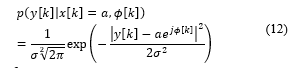
For transmissions like quadrature amplitude modulation (QAM), which relies heavily on signal amplitude and phase shifting in its transmission, noise can significantly impact its performance, specifically on its BER. A small amount of noise can incorrectly categorize the transmitted data. This error is especially apparent in optical transmissions because most utilizing the orthogonal frequency division multiplexing scheme produces a high peak-to-average power ratio resulting in noise that can increase the BER in a transmission medium.

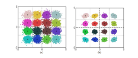
Figure 2: (a) 16-QAM constellation with high nonlinear phase noise; (b) with reduced noise [8]

Hence, solutions to addressing such nonlinearity are essential. In this work, two important techniques that work to that end analyze SVM and CAEM on how they affect optical fiber transmissions regarding their overall performance and fiber optic nonlinearity compensation. Performance comparison was made between the two using parameters of the different studies. In particular, the emphasis was on the use of coherent optical orthogonal frequency division multiplexing (CO-OFDM) or polarization division multiplexing using a 16-ary QAM (16-QAM) signal with varying fiber lengths and variables. The authors also propose a comparative index to fairly evaluate the two techniques based on the bit error rate (BER), power, and transmission distance. This paper is organized then as follows. Section 1 is followed by discussing the methods and a proposed comparative index in Section 2. Results and their discussions were done in Section 3, and recommendations given in Section 4.

2. Nonlinearity Compensation and Comparative Methodology

2.1. 16-QAM Least-Squares SVM Nonlinearity Equalizer

A 16-QAM CO-OFDM coupled with an SVM nonlinear equalizer is proposed in [2]. The optical fiber link is composed of multiple 100 km standard single-mode fiber (SSMF). Attenuation in the link is accounted for and compensated using Erbium-doped fiber amplifiers (EDFA). The ASE contributed by the EDFA is considered as white Gaussian noise. Inputs to the digital modulator are generated from a pseudo-random binary sequence (PRBS) module, which then undergoes the QAM modulation. An inverse fast-Fourier transform module is utilized to convert the time domain signal generated to an equivalent frequency domain. In this case, the pulses of the signal are kept ideal for simplifying the simulation. To maximize linear conversion between the OFDM signal and the optical field, the OFDM signal’s in-phase and quadrature segments are used by a pair of Mach-Zehnder modulators (MZM). Both MZM operates via push-pull configuration and is configured to be biased at the minimum transmission point to remove the chirp phenomenon effectively. Once the optical signal reaches the receiver after traversing N-span amplifiers, it is converted into an electrical signal by a 90⁰ photoreceiver. Noise due to the laser linewidth’s imperfections is disregarded as the study aims to isolate fiber nonlinearities due to other noise [2]. The signal then undergoes the normal decryption process before being fed into the machine learning algorithm, after which it is fully demodulated, and the error rate is calculated.

Figure 3: 16-QAM CO-OFDM SVM-NLE Diagram [2]

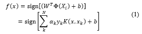
Support vector machines are powerful classifying tools yet can only be used as binary classifiers. Due to this restriction, this study’s approach combines multiple two-class SVMs for a multi-class model to be used. Since the study uses 16-QAM as its modulation technique, the signal is divided into sixteen (16) individual clusters in a constellation wherein each cluster represents data in a unique binary form [9]. For a single two-class SVM classifier, N pairs of vectors , k=1,…,N where  and y_k are the input and output patterns, respectively undergo training to obtain the hyperplane. y_k is the labeling function where y_k ∈ {1, -1}. Through this training process, possible noise in the constellation is distributed efficiently and accurately. Based on the training data present, SVM aims to construct a classifier f(x)

where  is the weight,  is the support vector,  is the bias term, and  is the mapping function. The training process determines the weight, support vector, and bias terms used for the constructed classifier. For more complex data to be accurately separated, a mapping function is used to transform the training data x_k into a higher dimension.  The SVM also utilizes a Kernel trick to help nonlinear decisions in mapping low complexity computations. The approach focused on this survey utilizes a radial basis function kernel in which only dot products are needed. K(x_i,k_j) ≡ exp (-ỿ_SVM||x_i – x_j||²)), ỿSVM > 0, with ỿ_SVM as the Kernel function.

Since there are more than two unique data sets to classify from in a 16-QAM constellation, the study employed a one versus rest rule, wherein a received data point would classify in a particular cluster if and only if it is accepted by that cluster and is rejected by the rest, if two or more clusters accept the data point then it is considered noise.

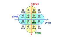
Figure 4: Implementation of a 4-level SVM to classify a 16-QAM constellation [10]

To further increase the SVM classification accuracy in noisier environments, the study opted to implement a least-square variant of the SVM studied in [11]. Least-Square SVM (LS-SVM) provides a more optimized solution using the following:

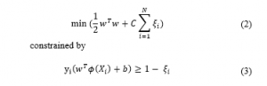
where  is termed as the slack variable which shows the error term which must satisfy the condition . C is known as the regularization parameter.

After the CD compensation process, both I and Q segments of the signal are fed into the LS-SVM in which the classifier is formed through a two-stage process of training and testing [2], [11].

1. Training
   • Arrange label , in-phase I and quadrature Q to format the SVM packet.
   • Select the RBF Kernel function and scale I, Q to [0,1]
   • Use cross-validation to determine the optimal C and ỿ_SVM
   • C and ỿ_SVM values to train the SVM.

2. Testing

• • Insert testing symbol.
  • Compare predicted labels to transmitted symbols to determine and evaluate the BER.

2.2. Code-Aided Expectation Maximization

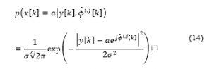
A wavelength-division multiplexing (WDM) and polarization division multiplexing (PolDM) system is considered in [12]. Nine simultaneously transmitting channels with the middle channel being the main focus of the study utilizes 16-QAM modulation with a 32 GBaud symbol rate. The optic signal goes through a 2640 km distance consisting of 33 spans of 80 km each. Dispersion-compensating fiber (DCF) is not utilized in the study; however, the same standard single-mode fiber (SSMF) is used for the fiber cable, and an erbium-doped fiber amplifier (EDFA) is employed to counteract fiber loss. The signal undergoes a chromatic dispersion compensation followed by a polarization demultiplexing at the receiver. A frequency estimation (FE) acts on the sampled signal to estimate the frequency with a margin of accuracy equal to or better than 4 MHz. A Viterbi algorithm compensates for any leftover frequency that utilizes an FIR filter length with phase averaging.

Due to noise correlating over time, traditional white noise assumption methods of demodulation are often suboptimal. The study in [12] partially compensates impairments done by both inter-channel and intra-channel nonlinear effects by exploiting the correlation of the phase noise through the use of CAEM. The phase noise correlation is dealt with by using a regularizer in the utility function of the algorithm. The CAEM describes as follows:

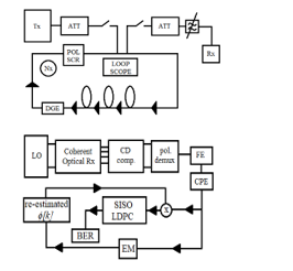
Figure 5: 16-QAM PDM CAEM Algorithm Diagram [12]

1. will be set as the th symbol after phase noise compensation in the th iteration between the EM and forward error correction (FEC) process .  and  are set as initial values.
2. The log-likelihood-ratio (LLR) is computed for each bit based on . Let be the th bit. The LLR is defined as follows if M-ary modulation is utilized.

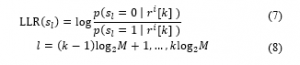
It is assumed that the residual noise in  patterns itself in a circularly symmetric zero-mean white Gaussian distribution. Constellation points whose labels are  are defined in the set  and likewise for .

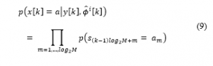
3. An updated log-likelihood ratio is obtained by decoding a soft-input-soft-output (SISO) FEC based on the initial .  bits are then converted to probabilities. Assuming a constellation point,  is labeled as a logarithmic bit sequence  we obtain:

4. The utility function is then setup – Expectation Step.

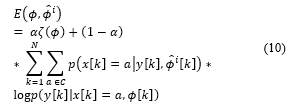
where N is the total number of symbols,  is the BER optimization weight with  The regularizer function  is described as follows:

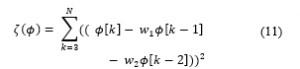
where  and  are the noise AR analysis weights. The expression  is computed as follows:

in which  is the noise variance that can be empirically computed with the aid of the training data.

5. The vector is calculated assuming the below conditions – Maximization step:

where  is the estimated phase noise between FEC and EM in the th iteration and the estimated noise between the E and M steps in the th iteration. To numerically compute for  a gradient-ascent method is used.

6. The utility function is recomputed, however instead of using (step 3), the following is used.

7. Step 6 is repeated until converges after which  is set.
8. Steps 1 to 7 are repeated until converges, and  being the final phase noise is estimated.

2.3. Simulation Parameters

The following tables show the parameters and conditions of each approach.

Table 1: Least-Square SVM Parameters Multiplexing CO-OFDM Distance up to 1200 km Amplifier EDFA Noise Figure 6 dB Fiber SSMF Span Length 100 km Attenuation Coeff 4.605 x 10-5 m-1 * Dispersion Coeff 17 ps/(nm · km) Nonlinear Coeff – EDFA Emission Factor – Symbol rate 40 Gbaud Tx & LO Linewidth – Modulation 16-QAM Sampling rate –
Table 2: Code-Aided EM Parameters Multiplexing PDM Distance 2640 km Amplifier EDFA Noise Figure – Fiber SSMF Span Length 80 km Attenuation Coeff 4.8354 x 10-5 m-1 Dispersion Coeff 17.025 ps/(nm · km) Nonlinear Coeff 1.3 (W · km)-1 EDFA Emission Factor 1.7741 Symbol rate 32 Gbaud Tx & LO Linewidth 100 kHz Modulation 16 QAM Sampling rate 1 sample/symbol

3.       Comparative Index, Results, and Discussions

The tables below show the results of each study’s approach. Since comparison is to be done using the BER, findings with Q-factor results were converted to their equivalent BER using the following [13]:

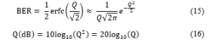
where Q is the Q-factor and erfc () is the complementary error function. Since the (erfc) used in calculating BER is approximated, any BER values computed will be approximations. To ensure the calculations’ high accuracy, BER values are displayed, having values up to seven decimal places.

3.1. Proposed Index

The authors proposed an index (17), which is a measure of how well each technique compares to others depending on the application. The index in Table 8 is calculated as follows:

(17)

Table 3: Quality Factor (dB) for 1000 km and 1200 km fiber length at differing Launch Powers [2] Launce Power Distance (km) 1000 1200 -3 dBm 9.50 8.90 -4 dBm 10.20 9.55 -5 dBm 10.40 9.95 -6 dBm 10.30 9.90 -7 dBm 10.00 9.60 -8 dBm 9.50 9.10 -9 dBm 8.90 8.50
Table 4: BER for 1000 km and 1200 km fiber length at differing Launch Powers. Launce Power Distance (km) 1000 1200 -3 dBm 0.0015509 0.0029533 -4 dBm 0.0006563 0.0014644 -5 dBm 0.0005011 0.0009053 -6 dBm 0.0005743 0.0009635 -7 dBm 0.0008500 0.0013820 -8 dBm 0.0015509 0.0024036 -9 dBm 0.0029533 0.0043513

Table 5: BER at Launch Power = -6 dBm for different fiber lengths

Distance (km)	Launch Power	Q-factor (dB)	BER
400	-6 dBm	11.50	0.0000909
600	-6 dBm	11.25	0.0001389
800	-6 dBm	10.90	0.0002423
1000	-6 dBm	10.30	0.0005743
1200	-6 dBm	9.90	0.0009635

3.2. LS-SVM Results

The BER values in Table 3 are extrapolated from the graphical results in [2], while BER values in Tables 4 and 5 are calculated estimates from the data of [2] using (15) and (16).

3.3. CAEM Results

The Q-Factor values in Table 6 are extrapolated from the graphical results in [12]. BER values are calculated estimates using (15) and (16) based on the Q-Factor.

Table 6: Q-Factor (dB) and BER as a function of Launch Power at 2640 km fiber length   Launce Power Distance (km) Q-Factor (dB) BER -2 dBm 2640 4.6 0.0555459 -1 dBm 2640 8.5 0.0043514 0 dBm 2640 11.4 0.0001081 1 dBm 2640 13.1 0.0000033 2 dBm 2640 6.9 0.0155732

3.4. Comparative Results

Table 7 shows BER values attained from the different studies under highly similar conditions, thus making it possible to compare their results. LS-SVM can be compared under a -6 dBm launch power at 1200 km fiber length while CAEM has results at 0 dBm launch power with a 2640 km fiber length.

Table 7: BER values under similar attributes

Algorithm	Distance (km)	Fiber Link	Launch Power	BER
LS-SVM	1200	–	-6 dBm	0.0009635
CAEM	2640	–	0 dBm	0.0001081

Table 8: Results Based on the Proposed Index

Algorithm	BER	Power   (Watts)	Distance (km)	Index
LS-SVM	0.0009635	0.0002512	1200	0.0031963
CAEM	0.0001081	0.0010000	2640	0.0000409

Low index values mean better overall performance for the algorithm. As shown in Table 8, the LS-SVM can be applied well in midrange haul and low complexity applications, whereas CAEM for long haul and high complexity optical networks.  The index provided in (17) for measuring and comparing the performance in the studies [12], [2] is thus proposed for nonlinearity compensation performance comparisons. Nonetheless, it also recognized that multiple values should be considered and further simulated to get graphical representations of the results.

4. Recommendations

Based on the results, LS-SVM provides nonlinearity compensation in a CO-OFDM 16-QAM system, but for longer fiber lengths, CAEM provides a significantly lower BER value. These outcomes make CAEM a preferred choice when it comes to long haul optical transmissions. Complexity wise it is recommended to utilize LS-SVM. CAEM is preferred despite the higher complexity due to its significantly lower index. One potential future work is to verify the results in an experimental setup.

Conflict of Interest

The authors declare no conflict of interest.

Acknowledgment

De La Salle University is acknowledged for supporting this work.

1. K. Kikuchi, “Fundamentals of Coherent Optical Fiber Communications,” Journal of Lightwave Technology, 34(1), 157–179, 2016. doi: 10.1109/JLT.2015.2463719.
2. T. Nguyen, S. Mhatli, E. Giacoumidis, L. V. Compernolle, M. Wuilpart, and P. Mégret, “Fiber Nonlinearity Equalizer Based on Support Vector Classification for Coherent Optical OFDM,” IEEE Photonics Journal, 8(2),. 1–9, 2016, doi: 10.1109/JPHOT.2016.2528886.
3. D. Semrau et al., “Achievable information rates estimates in optically amplified transmission systems using nonlinearity compensation and probabilistic shaping,” Opt. Lett., 42(1), 121–124, 2017. doi: 10.1364/OL.42.000121.
4. D. Lavery, D. Ives, G. Liga, A. Alvarado, S. J. Savory, and P. Bayvel, “The benefit of split nonlinearity compensation for single channel optical fiber communications,” in 2016 IEEE Photonics Conference (IPC), 2016, 799–802, 2016. doi: 10.1109/IPCon.2016.7831073.
5. H. Hu et al., “Fiber nonlinearity compensation of an 8-channel WDM PDM-QPSK signal using multiple phase conjugations,” in OFC 2014, 2014, 1–3, 2014. doi: 10.1364/OFC.2014.M3C.2.
6. G. P. Agrawal, “Nonlinear Fiber Optics,” in Nonlinear Science at the Dawn of the 21st Century, Berlin, Heidelberg, 195–211, 2000.
7. R. Dar, M. Feder, A. Mecozzi, and M. Shtaif, “Accumulation of nonlinear interference noise in fiber-optic systems,” Opt. Express, 22(12), 14199–14211, 2014. doi: 10.1364/OE.22.014199.
8. T. Pfau, S. Hoffmann, and R. Noé, “Hardware-Efficient Coherent Digital Receiver Concept With Feedforward Carrier Recovery for $ M $-QAM Constellations,” Journal of Lightwave Technology, 27, 2009, doi: 10.1109/JLT.2008.2010511.
9. E. Giacoumidis et al., “Kerr-induced nonlinearity reduction in coherent optical OFDM by low complexity support vector machine regression-based equalization,” in 2016 Optical Fiber Communications Conference and Exhibition (OFC), 2016, 1–3, 2016.
10. D. Wang et al., “Nonlinear decision boundary created by a machine learning-based classifier to mitigate nonlinear phase noise,” in 2015 European Conference on Optical Communication (ECOC), 1–3, 2015. doi: 10.1109/ECOC.2015.7341753.
11. C.-C. Chang and C.-J. Lin, “LIBSVM: A library for support vector machines,” ACM transactions on intelligent systems and technology (TIST), 2(3),. 1–27, 2011, doi: 10.1145/1961189.1961199.
12. C. Pan, H. Bülow, W. Idler, L. Schmalen, and F. R. Kschischang, “Optical Nonlinear Phase Noise Compensation for 9×32 -Gbaud PolDM-16 QAM Transmission Using a Code-Aided Expectation-Maximization Algorithm,” Journal of Lightwave Technology, 33(17), 3679–3686, 2015, doi: 10.1109/JLT.2015.2451108.
13. W. Freude et al., “Quality metrics for optical signals: Eye diagram, Q-factor, OSNR, EVM and BER,” in 2012 14th International Conference on Transparent Optical Networks (ICTON), 1–4, 2012. doi: 10.1109/ICTON.2012.6254380.

(Click Here)

(Click Here)