1. Introduction

In recent years, study and development of autonomous driving has been conducted in the automobile industry, IT companies, and universities in each country. In study on autonomous driving, some autonomous driving systems that combine Artificial Intelligence (AI) and model-free control methods is proposed [1,2]. However, it is considered that such the autonomous driving system is difficult to obtain system stability and reliability in unknown environments. Therefore, fusion technology of AI technology and model-based control has gained much importance in study on autonomous driving [3,4]. Model-based control is a control method in which a control target is represented by a mathematical model and optimal control input is determined based on the model. Model-based control is widely used in various industries [5]. It has problem that the control performance cannot be exhibited when the model is different from the actual dynamics. Additionally, the more complex the controlled object, the more complex the model and the more the amount of calculation. There is a limit to the number of computing units that can be equipped in an autonomous vehicle. Therefore, the model used for autonomous driving is required to be a simple model with less calculation amount. This paper proposes a simple and highly accurate method for vehicle identification (partially published in [6]).

Several studies agree that simple models, such as Kinematic Bicycle Model [7] and linear single-track model [8], are easier to design controllers for autonomous driving systems [9,10]. These vehicle models do not include nonlinear characteristics due to road conditions and driving conditions (environmental disturbances: road friction coefficient, large steering, acceleration, sideslip, etc.). Hence, the accuracy may be deteriorated due to a modeling error between the actual vehicle and the vehicle model. In order to consider the nonlinear characteristics of the vehicle, vehicle models that includes model equations such as tires and suspensions in the vehicle model has also been proposed [11,12]. However, since these vehicle models include multiple models expressions in the vehicle model, the structure of the vehicle model is complicated. It is inferred that if these are used in an autonomous driving system, it may impose calculated load on the computing unit and impair the real-time performance of the system. In other words, it is important for the vehicle model used for autonomous driving controllers to accurately model the vehicle in real time, even if there are environmental disturbances. This paper proposes a vehicle model based on the Kinematic Bicycle Model [7] in order to represent vehicle behavior simply and with high accuracy. The Kinematic Bicycle Model does not include nonlinear characteristics due to acceleration and deceleration or large steering, etc. Therefore, an error may occur between the actual gravity center position of the vehicle and the gravity center position calculated by the vehicle model. The behavior of the actual vehicle and the behavior calculated by the model are different due to the position error of the center of gravity, and the modeling error becomes large. Therefore, this method considers the vehicle model in which the center of gravity is fixed at the center of the wheelbase of the Kinematic Bicycle Model and the modeling error is expressed by the deviation of the front wheel steering angle. In addition, this study uses Neural Network to adaptively identify vehicle model by training and estimating the deviation. This paper verifies the usefulness of the proposed method through simulation experiments using vehicle motion analysis software (CarSim: Virtual Mechanics). In this study, simulations were performed in situations closer to actual driving conditions than in [6] (Section 4). Since this method models the vehicle while determining the control input in real time, it does not exist as a modeling technology alone and must be combined with model-based control. This paper shows an example using Model Predictive Control (MPC) as an example of model-based control to show the usefulness of the method. The method requires accurate location information acquisition. Since it is expected that the measurement accuracy will improve with the development of GNSS (Global Navigation Satellite System) in the future, the simulation is performed assuming that accurate position information can be obtained.

In summary, there are two aspects of the proposed approach that are particularly unique. The first is that the structure of the model is simple and easy to identify. In conventional models, several parameters must be identified in advance, but only one parameter is required in this study in advance. This means that the controller design of autonomous driving could be simplified by relieving the task of examining cornering stiffness and tire parameters in advance. Second, by focusing on the coordinates of the center of gravity, the approach can analyze the entire vehicle as nonlinear motion. Online learning may be able to respond to changes in vehicle mass (due to the number of passengers and loads) and road surface. It is notable that the method is robust to environmental disturbances and easy to identify.

This paper sets up the issue in Section 2. Section 2.1 introduces the conventional method and Section 2.2 describes our proposed identification method in detail. This paper also presents and discuss the simulation results in Sections 3 and 4. Section 3 mainly considers the effects of acceleration, deceleration and steering on the vehicle’s nonlinear characteristics, while Section 4 considers the situation with road surface changes. And Section 5 concludes this paper.

Figure 1: Kinematic Bicycle Model on the XY coordinate

2. Statements of The Issue

This section will set the issue for the proposed method. Section 2.1 introduces simple two-wheel models and accurate nonlinear models to clarify the problem. Section 2.2 details the proposed method for solving the problem.

2.1. Conventional study of vehicle models

2.1.1. Two-wheel model with simple structure

Typical vehicle models used for model-based control include simple two-wheeled models such as the Kinematic Bicycle Model [7] and linear single-track model [8]. These vehicle models are based on the assumption that the state quantities are observed instantaneously, and some conditions (e.g. constant speed, left and right tire characteristics are equal, roll and pitching motions are ignored) are set to represent vehicle dynamics in a simplified way. These vehicle models have simple structure, and thus the turning radius can be easily calculated. Therefore, they can be easily introduced to the controller design of autonomous driving systems. However, these do not take into account various nonlinear characteristics due to environmental disturbances (road friction coefficient, large steering, acceleration, etc.), which can cause modeling errors between the actual vehicle and vehicle models. This paper uses the Kinematic Bicycle Model as an example of the simple two-wheel model to test its accuracy. The model diagram of the Kinematic Bicycle Model is shown in Figure 1. Equations (1-4) show the model equations of the vehicle model. The velocity (m/s) and the front wheel steering angle (rad) are inputs, and the center of gravity coordinates of the vehicle model , the direction of the vehicle model (rad), and the sideslip angle around the center of gravity (rad) are outputs.  is the coordinates of the center of gravity observed one step ago.

here  is the current time,  is the sampling time, (m) are the distance from the front (rear) wheel axle to the center of gravity, and (m) is the wheel base.

The trajectory of the vehicle model without these nonlinear characteristics (Figure 1) is confirmed. In this case, experiments and verifications should be performed using actual vehicles, but verifications are performed by simulation experiments that are easy to analyze and verify and that can accurately acquire the vehicle state. Specifically, this study used the Driving Simulator in Figure 2. The Driving Simulator is a Windows PC with a vehicle motion numerical analysis software (CarSim) and a game handle device (Logitech) connected. The PC used in the simulation are as follows: Windows10 64bit, CPU: Intel(R) Core(TM) i7-9700 CPU @ 3.00GHz, and installed memory (RAM):8GB.

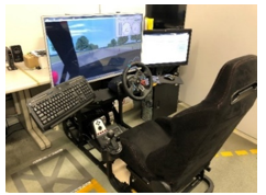
Figure 2: Driving Simulator

A simulation course [Slalom] was created on CarSim as shown in Figure 3. The driver drove this course between two pylons lined up in the course, gradually increasing the velocity as shown in Figure 5. The running trajectory at that time is the solid line in Figure 4 (Vehicle’s running trajectory). The velocity  obtained as the vehicle data at that time is shown in Figure 5, and the front wheel steering angle  is shown in Figure 6. The velocity  and the front wheel steering angle  are input to the vehicle model (1-4) and the running trajectory is calculated as shown by the broken line in Figure 4 (Equation of Vehicle Model). Figure 7 shows the position error between the observed trajectory   and the trajectory calculated by the vehicle model . From Figure 4 and Figure 7, there is a maximum position error of about 0.15m in the running trajectory of the actual vehicle and the running trajectory calculated using the vehicle model of (1-4). This is thought to be due to the nonlinear characteristics (tire deformation, expansion and contraction of suspension, etc.) caused by acceleration, deceleration and steering during running. It is consider that the front wheel steering angle  and the vehicle traveling direction do not match due to the influence of the nonlinear characteristic. This deviation affects the modeling error. In addition, this simulation is based on the assumption of asphalt surface. If it is snow or ice road, the deviation increases further. This is because the effect of the road surface is not taken into account in this model.

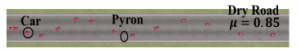
Figure 3: Simulation course［Slalom］

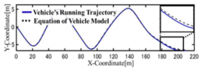
Figure 4: Driving trajectory

Figure 5: Velocity

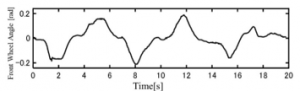
Figure 6: Front wheel steering angle

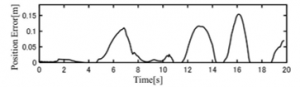
Figure 7: Position error

• Example of non-linear vehicle models that accurately represents vehicle behavior

 As shown in 2.1.1, simplifying the vehicle behavior may increase the modeling error. Hence, there are several conventional studies that use nonlinear vehicle models to represent the nonlinear motion of vehicles in detail. In literature [13], an autonomous driving system combined with a nonlinear vehicle model and MPC is proposed. The nonlinear model is a combination of two-wheel model and nonlinear tire model. This literature shows good results even on compacted snow surface with a low coefficient of friction. In this literature, two tire models were prepared beforehand, one for asphalt and the other for compacted snow, and were tested on each surface. In other words, the experiment is based on the assumption that the road friction coefficient is known. This means that the road friction coefficient, which changes from time to time, must be known.

To solve these problems, a combination of adaptive Model Predictive Control and tire-stiffness estimator [14] has been proposed [15]. This method estimates the tire stiffness from the tire-stiffness estimator. It is able to estimate tire stiffness in situations where the road surface changes and select the optimal road friction coefficient and tire parameters. However, the relationship between the chosen parameters and tire stiffness must be known. In order to find out the relationship between the two, it is necessary to conduct field tests or using a testbench beforehand, which may change depending on the degree of tire wear and other factors such as ageing. In addition, these literatures focused only on tire nonlinearity and did not mention nonlinear vehicle motion due to changes in vehicle mass (due to the number of passengers and loads.), suspension, body stiffness and other effects. These nonlinear motions can also lead to modeling errors. This paper proposes a vehicle model for online learning of nonlinear characteristics of the vehicle by focusing on the change of the vehicle’s center of gravity position. By focusing on the change of the center of gravity, it is possible to model not only the tires but also the nonlinear characteristics of the entire vehicle. Furthermore, online learning eliminates the hassle of pre-testing and allows you to deal with disturbances such as vehicle mass that change with each drive

• Vehicle Model to Estimate Modeling Error

As described in Section 2.1.1, due to the nonlinear characteristics of automobiles, deviation occurs between the front wheel steering angle  and the actual running direction of the vehicle. The actual direction of travel of the vehicle is defined as the front tire steering angle . Here, the front wheel tire steering angle  is an angle that includes nonlinear characteristics due to environmental disturbances and vehicle dynamics. The front wheel steering angle  is the angle that the front wheels are facing, which can be calculated by the steering wheel angle . In order to accurately represent the behavior of the vehicle, it is necessary to include in the vehicle model the deviation between the direction the front wheels are facing and the direction the vehicle is actually going, in other words, the deviation between the front wheel steering angle  and the front wheel tire steering angle . However, it is difficult to directly observe and theoretically obtain the deviation. Therefore, this deviation is named the modeling error  and is defined as the front tire steering angle  as (5).

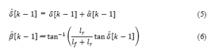
Since the front wheel tire steering angle  is defined as the actual direction in which the vehicle is traveling, (4) is modified as in (6). In other words, our proposed vehicle model is (1-3,5,6). The vehicle model is as shown in the Figure 8. The vehicle model needs to identify the distance from the front (rear) wheel axle to the center of gravity . The position of the vehicle’s center of gravity changes from moment to moment during driving. This is because acceleration, deceleration and large steering causes nonlinear motion in the vehicle, including the tires and suspensions. It is difficult to determine the exact position of the vehicle’s center of gravity. Therefore, in this study, the position of the center of gravity of the vehicle is fixed at the center of the wheelbase ( , and the identification error of the center of gravity position is corrected by .

Figure 8: Vehicle model including modeling error

Here, a method for estimating the modeling error  is described. Since the modeling error  is the parameter representing nonlinear motion due to acceleration and deceleration, steering, and road surface changes, it has nonlinearity and is expected to change from moment to moment. Therefore, this study proposes the method for estimating the model error  in real time while deriving the control input by model-based control.

This paper considers the system that uses MPC to derive the front wheel steering angle  and velocity  that are control inputs. MPC is a control law that derives the optimal control input while predicting its future behavior using a predictive model representing the dynamics of a control object. MPC solves an open-loop optimal control problem from the current time to finite horizon for each control period. MPC is an attractive method for controlling autonomous vehicles because it can consider the dynamics and constraints of the controlled object and the ability to adapt to driving scenarios [16-18]. Figure 9 shows the system configuration.

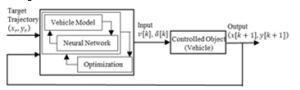
Figure 9: Block diagram of the proposed system

This system uses a Neural Network to train online the nonlinear characteristics of a vehicle that cannot be considered in the vehicle model. The trained Neural Network is used to control the vehicle while estimating the unknown parameters of the vehicle model. Figure 10 shows the flowchart of this system.

Figure 10: Flowchart of the adaptive identification method for vehicle

The control goal of MPC is to derive the control input that matches the output with the target trajectory. The control objective is to derive the control input (  and ) that matches the output  with the target trajectory . This system derives control inputs that minimize the cost function (7).

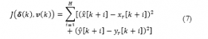
 is the prediction horizon. The prediction model (Vehicle Model and Neural Network in the Figure 9) predicts the vehicle trajectory . Since the trajectory depends on the future input, the input sequence  are derived so that the predicted trajectory  approaches the target trajectory  of the obtained input sequence, only the first  are used as the actual inputs.

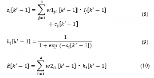
From here, the Neural Network that trains and estimates the modeling error  is described. From Figure 4 to Figure 6, it can be confirmed that the position error (modeling error) increases as the velocity  increases and the front wheel steering angle  increases. In other words, the position error is considered to depend on the velocity  and the front wheel steering angle . The parameter required to correct this position error is the modeling error . This modeling error  is considered to include nonlinearity. This study uses a 3-layer Neural Network with 2 inputs and 1 output for estimation. This is because the nonlinear system is modeled with high accuracy and the load on the computer memory is reduced as much as possible. The relationship between the input and output of the Neural Network is shown in (8-10). In this paper,  and  are inputs, –  are thresholds, and  and  are weighting factors. The input value of the hidden layers are – , and the sigmoid function is used for the output value –  of the hidden layers. Akaike’s Information Criterion (AIC) is used to determine the number of hidden layers. The input  is the front wheel steering angle  and the velocity , and the output  represents the modeling error .

      The observed values of the position coordinates are given to the Neural Network as instruction signal, and online training is performed so as to minimize the cost function (11).

Figure 11: Construction of the Neural Network

 represents the position coordinates of the vehicle model, and  represents the position coordinates of the actual vehicle.  represents the window width. This neural network is trained so that the position coordinates of the vehicle model  from  to  match the position coordinates of the actual vehicle . Altogether, the parameter , which represents the nonlinear properties, is estimated from the position coordinates.

     By training and estimating the modeling error due to the nonlinear characteristics online, the behavior of the vehicle can be accurately represented in situations such as acceleration and deceleration, large steering and road surface changes. Because the vehicle is identified in real time, it may be able to respond to changes in vehicle weight, such as changes in the number of passengers. Furthermore, our identification method only uses the wheelbase  as the setting parameter of vehicle model. This means that different types of vehicles can be identified by only changing the wheelbase . Conventional vehicle models have set parameters (e.g., cornering stiffness, vehicle mass, etc.), which vary for each vehicle. The key feature of this method is that there is only one configuration parameter.

3. Simulation of Fixed Road Surface

In this section, a simulation comparing the Kinematic Bicycle Model (1-4) with the proposed model (1-3,5,6) is described. As in Section 2, the simulation was performed using CarSim installed in the Driving Simulator. It verified whether the center of gravity coordinates of the proposed vehicle model  matches the center of gravity coordinates of the actual vehicle .The Kinematics Bicycle Model (1-4) and the proposed vehicle model  (1-3,5,6) were given the velocity  and front wheel steering angle  as inputs, and the trajectory was calculated. The accuracy is checked by comparing the calculated trajectory with the actual vehicle trajectory. The input data and the actual vehicle trajectory are obtained by driving the simulation course shown in Figure 3, which was created in the Driving Simulator (Figure 2) as a driving course with acceleration, deceleration, and steering. This study assumes that the 27 degree of freedom vehicle model in CarSim is the actual vehicle. This simulation assumes a dry asphalt surface (surface friction coefficient ?＝0.85) and drive a B-Class hatchback vehicle (Figure 12).

The driver repeatedly accelerated and decelerated between the two pylons in the course [Slalom] shown in Figure 3. Figure 13 and Figure 14 show the  and .The solid line in Figure 15 shows the running trajectory. In this paper, the trajectory is used as the actual vehicle trajectory. The dashed lines in Figure 15 show the trajectory when the velocity  ( Figure 13) and the front wheel steering angle  (Figure14) were given as inputs to the proposed model. The front wheel tire steering angle  is shown in Figure 16. The calculated position error between the calculated trajectory and the actual vehicle trajectory is shown in Figure 17 and the estimated modeling error  is shown in Figure 18. As shown in Figure 17, the maximum positional error is 0.05m, which is considered to be within the practical range.

Figure 12: B-Class hatchback vehicle in CarSim

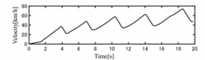
Figure 13: Velocity  （input）

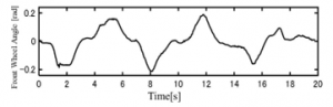
Figure 14: Front wheel steering angle  （input）

Figure 15: Driving trajectory［Slalom］

Figure 16: Front wheel steering angle  and front wheel tire steering angle

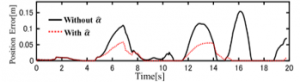
Figure 17: Position error

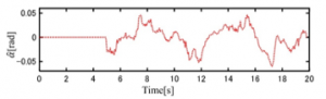
Figure 18: Modeling error

The results show that the behavior of the vehicle can be identified with high accuracy. This means that the proposed model (1-3,5,6) can contribute to the controller design of autonomous driving systems using model-based control. However, at this stage, this study has only validated a single driver driving a B-Class hatchback in CarSim several times around the track in a simulation experiment and have obtained good results. In order to prove the effectiveness of the proposed method, it is necessary to conduct similar tests on various courses and vehicle models, and this is a subject for future study.

4. Simulation of Road Surface Change

This section presents additional examples of situations that more closely resemble actual driving situations in order to verify the usefulness of the proposed model. As in Section 3, the experiments were conducted using the Driving Simulator shown in Figure 2. The course used is shown in Figure 19. This course was designed to simulate a mirror burn. Mirror burn is a phenomenon in which the surface of the road is polished by the traffic and becomes very slippery at a part of the intersection. This course was driven by the vehicle (B-class hatchback) in CarSim. This course is designed to have surface friction coefficient μ=0.2 at the center of the intersection and μ=0.5 outside the center of the intersection. This simulation assumes driving on the left side of the road because it is based on Japanese roads. The trajectory of the vehicle on this course is treated as the center of gravity coordinates of the actual vehicle . In addition to vehicle dynamics, this simulation allows us to verify whether the vehicle can adapt to changing road conditions. The trajectory of the vehicle  while driving on the course is shown by the solid line in Figure 22. The dotted lines in Figure 20 to Figure 25 indicate the boundary of the surface friction coefficient. Figure 20 and Figure 21 show the  and .The solid line in Figure 22 shows the running trajectory. In this paper, the trajectory is used as the actual vehicle trajectory. The dashed lines in Figure 22 show the trajectory when the  (Figure 20) and  (Figure 21) were given as inputs to the proposed model. The front wheel tire steering angle  is shown in Figure 23. The calculated position error between the calculated trajectory and the actual vehicle trajectory is shown in Figure 24 and the estimated modeling error  is shown in Figure 25. As shown in Figure 24, the maximum positional error is 0.01m, which indicates that the proposed model is able to adapt to the changes in the road surface.

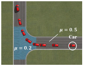
Figure 19: Simulation course ［Mirror Burn］

Figure 20: Velocity  （Input）

Figure 21: Front wheel steering angle  （Input）

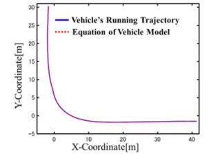
Figure 22: Vehicle’s driving trajectory ［Mirror Burn］

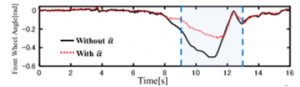
Figure 23: Front wheel steering angle  and front wheel tire steering angle

Figure 24: Position Error

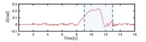
Figure 25: Modeling Error

5. Conclusion

The purpose of this paper is to identify an autonomous vehicle with high accuracy in real time. This paper proposed a simple vehicle model that represents the error in the center of gravity between the actual vehicle and the vehicle model as the deviation  of the front wheel steering angle. This paper also proposed the method to estimate the  in real time using neural network, and simulation experiments using CarSim showed the usefulness of the method in situations that require acceleration and deceleration, large steering, and road surface changes. The authors emphasize that the method can represent the nonlinear characteristics of the vehicle as it is learning online and that the only parameter to be identified in advance is the wheelbase. In other words, this study can eliminate the process of identifying multiple parameters beforehand and contribute to the design of control controllers that is robust to ever-changing environmental disturbances.

Conflict of Interest

The authors declare no conflict of interest.

1. M. Bojarski, D. Testa, D. Dworakowski, B. Firner, B. Flepp, P. Goyal, L. Jackel, M. Monfort, U. Muller and J. Zhang, et al. “End to end learning for self-driving cars.” arXiv preprint arXiv:1604.07316, 2016. https://arxiv.org/abs/1604.07316
2. F. Codevilla, M. Müller, A. López, V. Koltun and A. Dosovitskiy, “End-to-end driving via conditional imitation learning.” in 2018 IEEE International Conference on Robotics and Automation (ICRA), BNE, AU, 2018. https://doi.org/10.1109/ICRA.2018.8460487
3. B. Paden, M. Čáp, S. Yong, D Yershov and E. Frazzoli. “A survey of motion planning and control techniques for self-driving urban vehicles.” IEEE Transactions on intelligent vehicles, 1(1), 33-55, 2016. https://doi.org/10.1109/TIV.2016.2578706.
4. T Ariyoshi. “パーソナルカー 自動運転システムとそのめざす価値.” SICE 57(7), 488-492, 2018, in Japanese. https://doi.org/10.11499/sicejl.57.488
5. S.Adachi. “物理と情報と制御.” Calsonic Kansei technical review, 11, 6-14. 2014, in Japanese.
6. Y. Yamauchi,M.Saito and T. Ono “Adaptive identification method of vehicle modeling according to the fluctuation of road and running situation in autonomous driving”, 2019 58th Annual Conference of the Society of Instrument and Control Engineers of Japan (SICE), HIJ, JP, 2019. https://doi.org/10.23919/SICE.2019.8859845
7. R. Rajamani, Vehicle Dynamics and Control, ser. Mechanical Engineering Series. Springer, 2011.
8. R Bosch ”Automotive Handbook” 8 ed. John Wiley & Sons Ltd, 2011.
9. J. Kong, M. Pfeiffer, G. Schildbach and F. Borrelli. “Kinematic and dynamic vehicle models for autonomous driving control design.” in IEEE Intelligent Vehicles Symposium (IV), SEL, KR, 2015. https://doi.org/10.1109/IVS.2015.7225830
10. P. Polack, F. Altché, B. d’Andréa-Novel and A. Fortelle. “The kinematic bicycle model: A consistent model for planning feasible trajectories for autonomous vehicles?.” in IEEE Intelligent Vehicles Symposium (IV), SEA , USA, 2017. https://doi.org/10.1109/IVS.2017.7995816
11. K.Kabe and N. Miyashita” A study of the cornering power by use of the analytical tyre model.” Vehicle System Dynamics, 43(sup1), 113-122, 2005. https://doi.org/10.1080/00423110500139999
12. Y. Mitsuhashi and S. Fujii. “Validation of Fiala model for motorcycle with FEM tire model.( article in Japanese with an abstract in English)” Transactions of the Society of Automotive Engineers of Japan, 44(1), 75-80,2013. https://doi.org/10.11351/jsaeronbun.44.75
13. Y. Uno, R. Quirynen, S. Di Cairano, B. Karl. “Vehicle Integrated Control by Nonlinear Model Predictive Control in GNSS Based Autonomous Driving System.” IJAE, 50(4), 1176-1181, 2019, in Japanese. https://doi.org/10.11351/jsaeronbun.50.1176
14. K. Berntorp and S. Di Cairano, “Tire-stiffness and vehicle-state estimation based on noise-adaptive particle filtering,” IEEE Transactions on Control Systems Technology, 27(3), 1100-1114, 2018. https://doi.org/10.1109/TCST.2018.2790397
15. B. Karl, R. Quirynen, and S. Di Cairano. “Steering of autonomous vehicles based on friction-adaptive nonlinear model-predictive control.” 2019 American Control Conference (ACC), PA, USA, 2019. https://doi.org/10.23919/ACC.2019.8814448
16. F. Borrelli, P. Falcone, T. Keviczky, J. Asgari and D. Hrovat. “MPC-based approach to active steering for autonomous vehicle systems.” International journal of vehicle autonomous systems 3(2-4), 265-291 2005. https://doi.org/10.1504/IJVAS.2005.008237
17. M. Bujarbaruah, X. Zhang, H. Tseng and F. Borrelli. “ Adaptive mpc for autonomous lane keeping.” 14th International Symposium on Advanced Vehicle Control (AVEC), BJS, CN, 2018. https://arxiv.org/abs/1806.04335
18. X. Qian, I. Navarro, A Fortelle and F. Moutarde. “Motion planning for urban autonomous driving using Bézier curves and MPC.” in 2016 IEEE 19th International Conference on Intelligent Transportation Systems (ITSC), RIO, BR, 2016. https://doi.org/10.1109/ITSC.2016.7795651

(Click Here)

(Click Here)