1. Introduction

Most printing devices are constrained by a limited number of color Besides the FS, there are other algorithms that differ from this for intensities (typically 2/4/8/16 values), as consequence, before print- the weight distribution matrix. The error scattering technique is ing an image they must first convert the original color domain into a straightforwardly described in Algorithm 1.

new set of values that can be represented with the color intensities at their disposal. A process we call quantization.

Algorithm 1 Dithering algorithm An intuitive and trivial quantization method is to map each input

pixel to the nearest available color. However, most of the time this     ^{for rows ∈ image do}

for pixels p ∈ row do leads to a visually unpleasant and low quality output image due find closest color τ to p to a large number of artifacts. Here, dithering comes to help and ^{err = p −τ} diffuse err to neighbouring pixels according to the error diffusion scheme it has been proved to be able of achieving a higher quality results. end for In particular, the best known and popular dithering algorithms is ^{end for}

In case of binary dithering applied to a monotone image (e.g. grayscale to black and white), Algorithm 1 is just a simple threshold operation. Extending it to a larger set of colors (or tones) is a trivial change in finding the closest color. It was one of the most revolutionary methods and is widely used in digital printers, which prints small and isolated dots.

The other algorithms against which we will compare for the numerical experiments are: Atkinson, Burkes, Fan, Sieraa, Filter Lite, Jarvis, Judice and Ninke (JJN), Jarvis, Stucki and Shio Fan

[2].

There are several error distribution scheme and different ways to scan the image, such as the traditional left-to-right direction and the top-to-bottom raster. Considering all the matrices of weights related to the various methods would be redundant, therefore we show only a few in Figure 1 to clarify the concept.

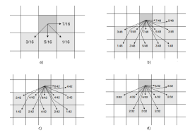
Figure 1: Error diffusion scheme for different dithering algorithms: Floyd-Steinberg

(a); Jarvis, Judice and Ninke (b); Stucki (c); Sierra (d). The flux of the whole image remains the same.

We also took care of the borders, in particular, we ensured that the image flux or average is maintained through the entire image, Figure 2 shows the modified FS error distribution weights in all particular cases.

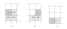
Figure 2: Error diffusion in the FS dithering in case of boundaries. a) first column, b) last column and c) last row.

The major shortcomings of the FS dithering algorithm are the generation of disturbing hysteresis artifacts or worm patterns at extreme gray-levels[3, 4] and the slowness [5].

2. Background and preliminaries

The purpose of image dithering, or halftoning, is the procedure that generates a pattern of quantized pixels able to create a continuoustone image illusion. A comprehensive analysis about halftoning techniques can be found in [2]. Dithering is necessary for showing gray scale images on printed surfaces when the only available tones are black and white. Dithering algorithms will produce different results with respect to quality and image characteristics. To allow a comparison between different algorithms, we must therefore quantify the performance. Doing so by means of psychovisual tests is hard due to the need of controlled conditions and long duration of the tests. A possible solution to this problem is developing quality measures that can numerically express the perceived visual difference between the dithered image and the original one. The ideal target would be to include several objective aspects of image quality within one single, robust and reliable measure, so to evaluate and improve dithering algorithms.

We cans also describe digital halftoning as an artifact minimization problem, because we search for the dithered image that minimizes the measured visibility of artifacts. We therefore need a computational model that allows us to compute the visible error, so to automatically rank images in an optimization algorithm. Nevertheless, measuring in a quantitative way the visual quality of a dithered image is still a challenging task.

Objective quality measures can be divided in two classes: mathematical/statistical ones and human visual system (HVS) based.

The first ones could be used to evaluate dithered patterns of constant grey values. These metrics provide a great understanding of the possible relationships for a given point distribution. These kinds of measures are usually independent of viewing conditions or observer, easy to compute thanks to the low computational complexity. It is possible to find in literature different examples of this kind of measures, such as: Structural Similarity (SSIM) [6], Peak Signal-to-Noise Ratio (PSNR) [7] and Mean Squared Error (MSE) [8]; nevertheless, none of these measures consider the presence of artifacts as explained in [9, 10].

The second one tries to model the perceived visual quality and predict artifacts generated by the dithering procedure. The ideal halftone algorithm is able to minimize this visibility. Since the eye detects more distortions at certain spatial frequencies, the development of a halftone visibility metric is based on a model of the HVS.

HVS models are relatively simple and have proven to be quite successful when applied to algorithms that seek the best possible distribution scheme. All digital halftone techniques, whether they are based on screening algorithms, error scattering or iterative halftone, all adopt these models, either explicitly or implicitly. In fact, even those methods that are categorized as model-free because they do not explicitly include an HVS block in their block diagram, still replace it with a low pass filter. Moreover, not only is an HVS model fundamental to the design of most halftone techniques, but additionally, the shape of the HVS model can be modified to achieve increased texture quality in the dithering result.

Therefore, the performance of a certain halftone algorithm can be maximized by adequately designing improved HVS models.

Digital halftoning usually refers to methods and algorithms able

to convert continuous-tone images to binary ones, for displaying them in bilevel devices such as printers, both ink jet and laser ones. Within the computer industry, the market demand for fast, high resolution printing devices has recently escalated. Halftoning’s contribution to this industry has been essential to its success. For this reason investigating image quality, and in particular finding an objective measure to evaluate the results is of fundamental importance.

2.1. A Quantitative Measure

As discussed, HVS models use human visual selectivity and sensitivity to model and improve the perceived image quality. HVS is based on the psycho-physical process that relates psychological phenomena (contrast, brightness, etc.) with physical phenomena (light intensity, spatial frequency, wavelength, etc.). It determines which physical configurations give rise to a particular psychological sensation (perceptual, in this case).

The two dimensional Discrete Fourier Transform (DFT) is applied on the image and then multiplied using Hadamard product with a Contrast Sensitivity Function (CSF), so that a component of the image at a particular angular frequency is weighted by the CSF value at that frequency. The result of this computation is the two dimensional DFT of an image that would lead to the same psychological response when viewed from a visual system with a flat CSF to which the original image leads when viewed by HVS [11]. The weighted signal-to-noise ratio (WSNR) of an M × N pixel binary image (y), given the original (x) of the same size is computed as:

where X(u,v), Y(u,v) and C(u,v) are correspondingly the DFT

of the input image, of the output image and the CSF.

2.2. Stochastic version

As already described in the previous sections, halftoning converts the input image into a black and white version of it to be reproduced on a binary output device, such as an ink-jet printer, which can only choose whether to print a dot or not in each position. The human eye, behaving as a low-pass filter, blurs the dots and spaces together and creates the illusion of many continuous shades of gray tones. Depending on the specific way the dots are distributed, a display device can produce different degrees of image fidelity with more or less granularity. According to the HVS, isolated and randomly arranged dots, if distributed in a proper manner, should produce images with the highest quality, maintaining fine details and sharp edges. Nevertheless, some displays and printing devices are unable to reproduce isolated dots consistently in their entirety and, as a result, introduce printing artifacts that greatly degrade the aforementioned details that the computed dot distribution is designed to preserve. For this reason, many printing devices create periodic patterns of grouped dots, which are easier to produce on the printed page in a consistent manner. For this reason, in our halftone study, the main objective is to determine the optimal dot distribution for that HVS, and then produce these models computationally efficiently.

Since the first article in which Floyd and Steinberg’s algorithm was mentioned, many changes to the original error spread algorithm have been introduced to avoid the undesirable artifacts present in the original algorithm. But while these modifications eliminate disturbing artifacts at certain levels of gray, many do so therefore at the expense of other levels. Jarvis [12] and Stucki [13], for example, introduced a different mask model and weights, called 12-element error filter, but the artifacts remain during the algorithm because of the fixed behavior manifested by these algorithms. Hence we realize that the problem is not related to the number of elements involved but rather to the determinism of the method. Other approaches suggested to change the scanning path in which pixels are processed, including the serpentine as the most trivial up to the space-filling curves like Hilbert’s curves. Unfortunately, these methods still create strong periodic patterns. To mitigate the problem of artifact our idea is to transform the FS algorithm, a deterministic algorithm, into a Stochastic (SFS) version inspired by [14]. A crucial point of our new approach is the preservation of the average image. As in all halftone methods, where everything and only the error is spread. Even in our method, while modifying the weight matrix at each pixel, the average of the values of the original image is not changed.

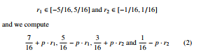
In particular we choose a real number p and, for each pixel, we generate 2 random number: r₁ ∈ [−5/16,5/16] and r₂ ∈ [−1/16,1/16] and we compute

as error diffusion coefficients. This method, as a modification of Ulichney’s one[15], is a good approximation of a blue-noise process. Blue-noise halftoning is characterized by a distribution of binary pixels where the minority pixels are spread as homogeneously as possible. This method of pixel distribution creates a pattern that is isotropic (or radially symmetric), aperiodic and does not contain any low-frequency spectral components. From the considerations made about HVS, it’s not surprising that blue-noise creates the visually optimal arrangement of dots. Unfortunately, blue-noise is not trivial or fast to generate [16], but whit our method this can be approximated.

2.3. Optimal choice of p

By introducing our new method we have underlined the need to choose a p parameter.

In our previous work the choice of p was totally empirical and not automated, that is, we tried different values of p in a predetermined range and picked the best according to the image quality measured by WSNR. Here we introduce a method for the automatic setting of p. As pointed out above, these algorithms are often used for printers in different areas, but often as an integral part of industrial processes. For this reason and for the sake of completeness, finding a fully automatic method would make the method more effective and usable on a large scale. There are two critical issues to be addressed: the choice of an appropriate interval and the need for an intervention by the operator for the choice. First of all, let’s discuss the choice of the interval. As we have defined p there are no limitations, it simply has to be a real value. Since it is not a probability, it can certainly assume both values greater than 1 and negative values. Conceptually there is a symmetry, at least on average, between negative and positive values so we can only take into account positive values without losing in the generality. On the other hand, choosing values much greater than 1 means to substantially change the coefficients of the matrix used for the diffusion of the errors, for

example choosing p = 2 the values, on average, are doubled. In addition to these preliminary considerations we conducted several experiments aimed at understanding where the maximum value of WSNR was in relation to the p choice. As it can be seen in Figure 3 , the maximum is usually included in the [0,2] interval.

Figure 3: Sample of the algorithm behaviour for p in the interval [0,2] for some images of the dataset available in [2]. Due to the stochastic nature of the algorithm, we repeat the algorithm 10 times with different random seeds for each value of p, plotting minimum, average and maximum value for the resulting WSNR.

Once the range is fixed, we address the second issue by means of an optimization algorithm that provides the p value that maximizes the WSNR. The first idea, given the amount of references in the literature, was to use a first-order technique as a gradient method [17]. But we immediately noticed that, due to the lack of convexity of the function to be maximized, such methods are often not effective. There are certainly techniques to use gradient methods even in non-convex areas but they require at least the differentiability of the function. Since we have to maximize a stochastic process we see both the basic hypotheses of the gradient methods fall: convexity and differentiability. Fortunately, our implementation of the parallel algorithm on GPUs makes execution time particularly low, even for large images. This allows us to approach efficiently the problem in an empirical way without increasing the time excessively. Considering all these premises, our final idea is to calculate, first, the WSNR for different values of p ∈ S _n where S _n is an equally spaced partition of the interval [0,2] with n elements. Due to the stochasticity of the method, for each p ∈ S _n we consider the average over m runs.

Finally, choose the p with the highest average WSNR. We summarize our method in the equation 3 where m is the number of runs, I and SFS(p) represent respectively the input image and the output image obtained from a single run of our stochastic dithering algorithm with parameter p.

We obtained the best results with the following configuration:

• Size of partition S _n, n = 100
• Number of repetitions for each p, m = 10

In this way, given any image in our experiments, the method lead to satisfying results in terms of similarity to the initial image.

3. GPU implementation

Dithering algorithm are infamously known for being ”embarassingly” unparallel due to the inherently sequential nature of the dithering operation: the every pixel output depends on all the previously computed outputs. Achieving good speed ups in such problems is a challenging task and several work from the research community tried to overcome this issue, either proposing a ”friendlier” dithering algorithm or a more efficient implementation. For example in [18]– [20] they introduce a block-based error diffusion algorithm which allows to simultaneously process blocks of pixels and produced good visual results, however is not clear which block dimension should be taken in order to get the best image quality; whereas in the work [21] the authors propose to parallelize over multiple pages in order to saturate the GPU utilization, in this work we focus on a single image case; in [22] they propose an efficient implementation that consists of a hybrid approach where CPU and GPU are both exploited but the CPU is used in the regions where GPU is expected to perform worse, in particular, towards image corners; finally [5] provided an optimal parallelization algorithm from a theoretical point of view, unfortunately, assigning each thread a diagonal portion of the image is currently not suited for general purpose devices as it causes more time spent for additional computational overhead than what parallel devices can manage to reduce.

In this work, we adopt the classical Floyd-Steinberg algorithm as it’s still the dithering algorithm that yields the best result and propose an implementation that rely solely on GPUs. Graphics Processing Units (GPUs), in particular General Purpose GPUs, are massively parallel architectures that comprises thousands of cores designed to compute in an extremely efficient way repetitive and simple operations such as those involved in the rendering pipeline in Computer Graphics, hence ”Graphics” in the name. Each core are less performing and simpler than state of art processors but the computational power in such devices lies in the number of cores rather than the capability of each single core. Nowadays GPUs are widely adopted for many tasks in data mining, physics simulation, medical imaging and machine learning, to name a few, hence the ”general purpose” in the name. We propose an implementation ^[1] that is optimized for the NVIDIA GPUs, from which we will also get the results reported in section 4.1, and we program with the architecture’s standard Application Programming Interface (API), called CUDA [23] developed by NVIDIA itself. Nonetheless, our implementation takes into account obstacles and design principles valid for almost all GPUs so it’s not limited to NVIDIA architectures.

Our implementation consists of two parallelization levels we call stream level and pixel level. First of all we, describe the pixel level parallelism consists of a function, named Parallel-FS, that implements the Floyd-Steinberg on GPU and assumes the image being already stored in the GPU memory, this function will be then invoked by the stream level function.

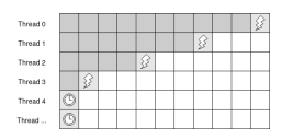
Figure 4: Each thread is assigned a row and waits for the previous one to be three pixels ahead instead of two. The thunder symbol on the diagonal represents the pixels processed simultaneously, whereas the clock indicates a waiting thread

In order to achieve good results one must take into account the of hardware on which the algorithm is executed. GPUs are SIMT (Single Instruction Multiple Thread) architectures partitioned in several Streaming Multiprocessors (SM), the latter are clusters of cores with multiple hardware schedulers for dispatching a fixed number of threads called warps. Each thread in the warp are committed to perform the same operation simultaneously, a feature called lock-step execution, and they are able to fetch multiple data at the same time if the addresses in the memory are aligned, a phenomena called ”coalesced access”. While these are good features in simple and regular memory accesses, it becomes actually a downside in case of FloydSteinberg because operations and accesses are neither simple nor regular. Dithering algorithm finds the closest color input and handle borders with many conditional, hence branching, instructions, which hurts the performance as the device must turn-off the portion of the threads not involved in the current branch because of the lock-step execution, moreover there’s no coalesced access as the error diffusion scheme follows an irregular pattern leading to increased latency. This is the reason why the optimal theoretical algorithms presented in [5] cannot be implemented, nonetheless we try to approximately recreate the theoretical optimal situation in Parallel-FS. The function takes as input three data structures, an input buffer I_{buf f} where the original image is stored, an output buffer O_{buf f} where the result will be stored and error buffer E_{buf f} for the temporary error diffusion values. Each row i is assigned a thread which, for each pixel

(i, j), j ∈ {1,…, I_WIDTH} where I_WIDTH is the image width, reads from the input buffer and computes the output O_{buf f} (i, j) by finding the closest color according to the value S = I_{buf f} (i, j) + E_{buf f} (i, j), and distribute the error S − O_{buf f} (i, j) to the neighbouring pixels according to the error diffusion scheme of Floyd-Steinberg, updating E_{buf f} (i, j+1), E_{buf f} (i+1, j), E_{buf f} (i+1, j−1) and E_{buf f} (i+1, j+1).

The actual implementation carefully takes into consideration also borders compared to this simplified formulation. Each thread must synchronize with the previous thread in order to compute the assigned pixel result, in our implementation, in order to avoid update conflicts in the error buffer, which would require slow atomic operations, each thread waits for the previous one to be three pixels ahead with respect to his row instead of two, similarly to [21] (see Figure 4). The Figure 4 also illustrates how pixels are processed simultaneously along the diagonal (hence the name ”pixel level parallelism”).

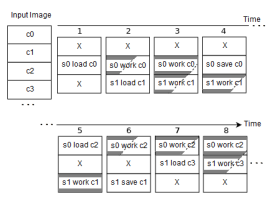
Figure 5: Visual illustration of the Double Buffering parallel execution scheme for the stream level parallelism, with two CUDA streams; sj and ci and denote CUDA stream respectively and image chunks. The ”load” and ”save” operations represent the data transfer from host to device input buffer I_{buf f} and from device output buffer O_{buf f} to host respectively and ”work” consist of the invocation of Parallel-FS. It can be noted that, starting from time step 2, the memory transfer latency is completely hidden by GPU activity. ”X” denotes the empty chunk, note that there is always an empty chunk because given N_STREAMS there are N_STREAMS + 1 blocks in the data structure, so each iteration, every stream finds the results of the first row of the error buffer already calculated by the previous stream by simply sliding up.

The stream level parallelism addresses a problem more related to the physical devices limitation rather than the FS algorithm. In previous function we assumed the image to be already when the output is ready, the result is transferred back into host memory. Unfortunately, in most parallel implementations memory bandwidth represents one of the main bottleneck. The outer loop in our stored in GPU memory, however, for a task to be executed on GPU, every required data must be copied first from host memory (accessible by CPU only) to device memory (accessible by GPU only) and parallel implementation addresses this problem by hiding almost completely the memory transfer overhead between CPU and GPU wit the double buffering technique, which also removes the device memory size constraint for huge images.

Given an image of size I_HEIGHT × I_WIDTH and two input parameters N_CHUNKS and N_STREAMS , the first parameter define the number of chunks the image is divided into, whereas the latter represents the number of chunk to be processed simultaneously. First we define

ChunkHEIGHT = NIHEIGHTCHUNKS and we divide the image into NCHUNKS of size Chunk_HEIGHT × N_WIDTH, secondly we create three data struc-

ture of size (ChunkHEIGHT · (NSTREAMS + 1)) × IWIDTH size for the input, output and error buffer respectively. Now, N_streams CUDA stream are created, each of these concurrent execution stream are assigned an image chunk are responsible of computing the result by invoking the Parallel-FS function previously described on the assigned chunk. During the algorithm execution, every function invoked by each stream references to the same data structure but on a different memory address offset, the size of each buffer is

N_STREAMS + 1 chunk blocks instead of N_STREAMS because the the additional chunk allows to leave one chunk empty at every iterative step so Parallel-FS function avoids storing the error computed in the last row into an auxiliary buffer, minimizing the number of conditional operations. Because of the empty chunk, when a CUDA stream finishes the job, it can slide on the upper chunk in a toroidal fashion along the height, which means that the errors computed in the last row of the data structure are actually propagated in the first and the CUDA stream working in the first block moves to the last in the next outer loop iteration as it finds the error values ready to be used. The indexing and synchronization required to ensure the overall correctness of the FS algorithm details will not be discussed for the sake of simplicity. The final result is that when some CUDA streams are processing their chunk, others are transferring data from host to device memory and vice-versa, thus the memory bottleneck is hidden and the architecture is fully exploited. In Figure 5 we show the presented parallel execution scheme.

3.1. Theoretical improvement

Consider an image of size P × Q, where P identifies the number of rows and Q the number of columns. We want to know the order of magnitude of the time that is theoretically needed to process the whole image. We use as a measure unit the time needed to process a single pixel.

In the serial version: Time = P × Q where Time is the time for the whole process. In the parallel version, with the same image dimension, we have

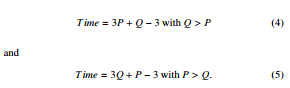
Considering, as said before, the time we use to process the single pixel we can assume to spend a M time to calculate the first row, but at this same time, always considering the parallel implementation, we have already calculated the triangle at the top left as shown in Figure 4. Going on to finish the second line, we only need to calculate another 3 pixels and we can proceed with a similar reasoning for all the rows in the image. So we have Q+3×(P−1) = Q+3P−3. Even in an image where the number of rows and columns is swapped we have the same runtime. For these considerations we can conclude that we pass from a time that grows as O(P × Q) with the input size, in the serial case, to a time that grows linearly O(P + Q) in the parallel case, all this from a theoretical point of view. This allows us to have a great saving in computational time, especially in industrial contexts where the images are of huge dimensions. This means an incredible acceleration, especially when the size of the image is large, as often happens in industrial cases.

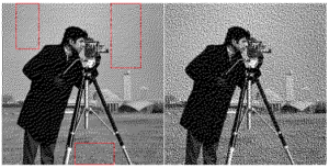
Figure 6: Cameraman image dithered with p = 0 on the left. The red rectangles highlight regions with visible artifacts. On the right, dithered image with optimal p value to maximize the WSNR value.

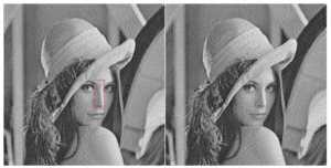
Figure 7: Lena image dithered with p = 0 on the left. The red rectangles highlight regions with visible artifacts. On the right, dithered image with optimal p value to maximize the WSNR value.

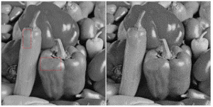
Figure 8: Peppers image dithered with p = 0 on the left. The red rectangles highlight regions with visible artifacts. On the right, dithered image with optimal p value to maximize the WSNR value.

4. Numerical experiments

The authors of [2] provided a sufficiently large dataset of images on which we applied our algorithm^[2], the Digital Halftone Database (DHD). This dataset is composed of 196 reference images extracted from the CVG-UGR-Image database and the Genreal-100 dataset. In addition to these real images, we also assessed our approach on synthetic images. In particular, a particularly complicated image to process is the grayscale gradient, as in the Figure 10 or multi-tone chessboard. Moreover, the well known Lena, peppers and cameraman have been tested as well. Not all the images have same values of width and height since the algorithm can be applied to rectangular pictures as well. In the first experiments, we chose synthetic images.

To verify the improvement with respect to the presence of artifacts, we applied our algorithm to images composed of all shades of the (0 − 255) grayscale. This was done because some tones are more susceptible than others to artifact forming. In a second experiment we applied the new techniques to images often used in published works, in order to compare the results with the literature. Finally we compare against the results of [2], that are provided as results images in the same dataset. Obviously it can be observed that there is a considerable difference between the proposed stochastic approach and the simple FS. The experiments were performed on a desktop computer equipped with a CPU and GPU with the following specifications: Intel i7 7700K CPU, NVIDIA GeForce GTX 1080 GPU and 32GB RAM.

4.1. Results

With respect to image quality, we computed the measure described in Sec. 2.1 after applying FS, SFS and, for completeness, other dithering algorithms known in literature: Stucki[13], SIERRA[24] and Jarvis, Judice, and Ninke [12]. The results for the different images in Figure 10 (top row) and Figure 6, 7 and 8 are shown in Table 1 were we highlighted in bold the best WSNR values. The charts in Figure 13 show the behaviour of the WSNR value with respect to p for these images. Furthermore, we provided additional visual comparisons in Figures 11 and 12.

We compared our algorithm to the error diffusion ones presented in [2] on the same DHD dataset previously mentioned. We computed WSNR from the output images that are made available in the dataset and compared against our approach: over 196 different images we achieved the maximum WSNR value amongst all the algorithms 71% of the times, while the remaining 29% has been topped by the Filter Lite Dot Diffusion algorithm from [25].

In Table 2 we report the values of WSNR for some images of the dataset. We have to remark that, due to the different output size of the image, for some pictures we were unable to compute the WSNR value of comparison. The algorithms that are taken into account here are our FSF, Atkinson (ADD), Burkes (BDD), Fan (FDD), tradirional Floyd Steinberg (FSDD), Frankie Serra (FSIDD), Filter Lite (FLDD), Jarvis Judice and Ninke (JJNDD), Jarvis (JDD), Stucki (SDD) and Shio Fan (SFDD).

In addition to providing a theoretical discussion, we tested the different versions of the algorithm, serial and parallel, on images of different sizes. As we expected we obtained very good results: while serial time increases quadratically, parallel time increases only linearly. Let’s better illustrate the trends in Figure 9.

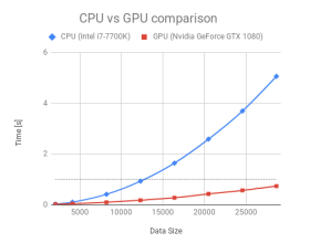
Figure 9: Comparison between the two versions: serial and parallel. Time in seconds on vertical axis, horizontally there is side dimension in pixels of a square image. In dotted line: all parallel execution time are less than one second.

Table 1: Dithering methods WSNR comparison

Image	FS		SFS		Stucki	Sierra	JJN
		p= 0.25	p= 0.5	p= 0.75
Gradient	52.58	53.15	53.34	53.28	50.49	50.64	50.28
Lena	48.51	48.48	48.57	48.51	41.79	41.58	41.08
Cameramen	45.78	46.02	46.30	46.43	39.29	39.13	38.61
Pepper	46.13	46.39	46.93	47.27	39.45	39.13	38.55

Table 2: Error Diffusion WSNR comparison

Index	FSF	ADD	BDD	FDD	FSDD	FSIDD	FLDD	JJNDD	JDD	SDD	SFDD
1	47.50	20.00	43.61	44.33	48.23	40.90	49.74	26.35	40.44	41.44	44.48
3	50.64	24.09	44.40	44.22	46.92	41.28	47.99	28.72	40.79	41.51	44.63
5	45.49	18.80	41.72	41.08	44.91	38.80	46.15	23.56	38.27	39.11	41.28
7	49.77	20.99	43.65	45.49	47.57	41.22	49.57	27.41	40.73	41.60	45.97
17	44.97	15.81	39.52	40.40	42.48	36.30	43.72	20.87	35.80	36.50	40.79

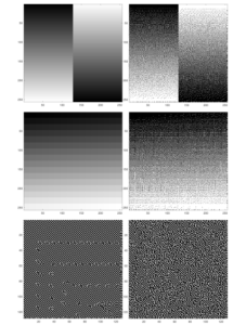
Figure 10: Inverted gradient pattern, original image (top-left) and halftoned using traditional FS (top-right): emerging artifacts are clearly discernible. In the middle row, 256 squares of all possible 1 Byte quantization values (left) ant their dithered version (right) Bottom line, particular of a single tone (value 128): on the left side artifacts arise distinctly with traditional FS, while on the right side the stochastic nature of the method allows no emerging pattern.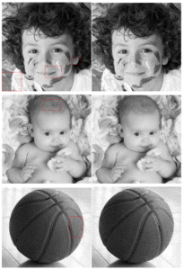

Figure 11: On the left: dithered images using FLDD for images 24, 4 and 6 of the Digital Halftone Database. The red rectangles highlight regions with visible artifacts. On the right, same images dithered using SFS with best p*.

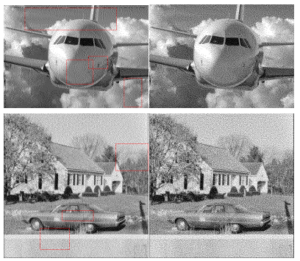
Figure 12: On the left: dithered images using FLDD for images 26 and 7 of the Digital Halftone Database. The red rectangles highlight regions with visible artifacts. On the

right: same images dithered using SFS with best p*.

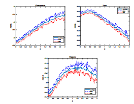
Figure 13: WSNR computed for our Stochastic Floyd-Steinberg algorithm with p ∈ [0,2] on the 3 well known images of Cameraman, Lena and Peppers. We proceed as for Figure 3.

5. Conclusions

In conclusion, the new algorithm we presented solves both the problems highlighted at the same time: the presence of artifacts and the slowness of execution. In particular, the transformation of the algorithm from deterministic to stochastic, with the introduction of a white noise, avoids the emergence of artifacts. The improvement can be evaluated through a specific measure that takes into account human perception called WSNR. Moreover, there is no increase in computational time; on the contrary, the parallel version we propose shows an excellent speed-up as the image size increases; which, especially in industrial applications, can be very large. Thanks to our parallel implementation, which guarantees speed to the method, we were able to fully automate the technique. So given an image we are capable of applying the best amount of stochasticity to the algorithm, thus obtaining an image as free of artifacts as possible. All the research part of the optimal parameter is done before the actual image printing process. This guarantees a method in which the operator does not have to make a decision and the printer is not occupied for a long time. In conclusion, the method is totally automatic, fast and guarantees a final image as close as possible to the initial one and suitable for printing. As future work some of the

possible extensions could be: more sophisticated methods to find optimal p, developing other error measures that take into account artifacts or geometric textures of different kinds. Another idea is to evaluate the 4, 8 and 16 gray tones versions of the dithering algorithm by proposing a technique that finds the best trade-off between image quality and number of tones.

1. R. W. Floyd, L. S. Steinberg, “An adaptive algorithm for spatial gray scale,” in Proceedings for the Society for Information Display, 75–77, 1976.
2. J. M. Guo, S. Sankarasrinivasan, “Digital Halftone Database (DHD): A Com- prehensive Analysis on Halftone Types,” in 2018 Asia-Pacific Signal and Information Processing Association Annual Summit and Conference (APSIPA ASC), 1091–1099, IEEE, 2018.
3. Z. Fan, R. Eschbach, “Limit cycle behavior of error diffusion,” in Pro- ceedings of 1st International Conference on Image Processing, volume 2, 1041–1045, 1994, doi:10.1109/ICIP.1994.413514.
4. M. Pedersen, F. Albregtsen, J. Hardeberg, “Detection of worms in error diffu- sion halftoning,” Proceedings of SPIE – The International Society for Optical Engineering, 7242, 2009, doi:10.1117/12.805555.
5. P. T. Metaxas, “Optimal Parallel Error-Diffusion Dithering,” in Proceedings of SPIE – The International Society for Optical Engineering, volume 3648, 485–494, doi:10.1117/12.334593.
6. P. Ndajah, H. Kikuchi, M. Yukawa, H. Watanabe, S. Muramatsu, “SSIM im- age quality metric for denoised images,” in Proc. 3rd WSEAS Int. Conf. on Visualization, Imaging and Simulation, 53–58, 2010.
7. A. Hore´, D. Ziou, “Image Quality Metrics: PSNR vs. SSIM,” in 2010 20th International Conference on Pattern Recognition, 2366–2369, 2010, doi: 10.1109/ICPR.2010.579.
8. B. Girod, “Psychovisual Aspects Of Image Processing: What’s Wrong With Mean Squared Error?” in Proceedings of the Seventh Workshop on Multidimen- sional Signal Processing, 207–220, 1991, doi:10.1109/MDSP.1991.639240.
9. T. Mitsa, K. L. Varkur, “Evaluation of contrast sensitivity functions for the formulation of quality measures incorporated in halftoning algorithms,” in 1993 IEEE International Conference on Acoustics, Speech, and Signal Processing, volume 5, 301–304, 1993, doi:10.1109/ICASSP.1993.319807.
10. D. R. Mehra, “Estimation of the Image Quality under Different Distortions,” International Journal Of Engineering And Computer Science, 8, 17291–17296, 2016, doi:10.18535/ijecs/v5i7.20.
11. R. Na¨sa¨nen, “Visibility of halftone dot textures,” IEEE Transactions on Sys- tems, Man, and Cybernetics, 14(6), 920–924, 1984, doi:10.1109/TSMC.1984. 6313320.
12. J. F. Jarvis, C. N. Judice, W. Ninke, “A survey of techniques for the display of continuous tone pictures on bilevel displays,” Computer graphics and image processing, 5(1), 13–40, 1976, doi:https://doi.org/10.1016/S0146-664X(76) 80003-2.
13. P. Stucki, “Image processing for document reproduction,” in Advances in digital image processing, 177–218, Springer, 1979.
14. R. Ulichney, Digital Halftoning, MIT Press, Cambridge, MA, USA, 1987.
15. R. Ulichney, Digital halftoning, MIT press, 1987.
16. I. Georgiev, M. Fajardo, “Blue-noise dithered sampling,” in ACM SIGGRAPH 2016 Talks, 1–1, 2016.
17. D. P. Bertsekas, J. N. Tsitsiklis, “Gradient convergence in gradient meth- ods with errors,” SIAM Journal on Optimization, 10(3), 627–642, 2000, doi: 10.1137/S1052623497331063.
18. Y. Zhang, J. L. Recker, R. Ulichney, I. Tastl, J. D. Owens, “Plane-dependent error diffusion on a GPU,” in Proceedings of SPIE – The International Society for Optical Engineering, 2012, doi:10.1117/12.906966.
19. Y. Zhang, J. L. Recker, R. Ulichney, G. B. Beretta, I. Tastl, I.-J. Lin, J. D. Owens, “A parallel error diffusion implementation on a GPU,” in Proceed- ings of SPIE – The International Society for Optical Engineering, 2011, doi: 10.1117/12.872616.
20. P. Li, J. P. Allebach, “Block interlaced pinwheel error diffusion,” Journal of Electronic Imaging, 14(2), 1–13, 2005, doi:10.1117/1.1900136.
21. B. Trager, C. W. Wu, M. Stanich, K. Chandu, “GPU-enabled parallel process- ing for image halftoning applications,” in IEEE International Symposium of Circuits and Systems (ISCAS), 1528–1531, 2011, doi:10.1109/ISCAS.2011. 5937866.
22. A. Deshpande, I. Misra, P. J. Narayanan, “Hybrid implementation of error diffusion dithering,” in 18th International Conference on High Performance Computing, 1–10, 2011, doi:10.1109/HiPC.2011.6152714.
23. Nvidia, “CUDA Programming Guide Version 10.0,” .
24. T. Helland, “Image Dithering: Eleven Algorithms and Source,” http://www.tannerhelland.com/4660/ dithering-eleven-algorithms-source-code/ [Accessed: Apr. 14, 2019].
25. C. Labs, “Libcaca study: the science behind colour ASCII art,” http://caca.zoy.org/wiki/libcaca/study/introduction [Accessed: Jul.20, 2020].

(Click Here)

(Click Here)