1. Introduction

This study shows new traffic congestion analysis in one of typical mega city in India. In general, it is hard to make traffic analysis especially in development countries where there is economical difficulty for infrastructure improvement under higher  demand of transportation by strong economic growth. Author has a chance to proceed traffic management system deploy in Ahmedabad city of Gujarat state of India since 2015 by Japan International Agency support program for the reduction of traffic congestion. The traffic management system consists of 14 traffic monitoring Cameras along their main streets and traffic condition indication by the 4 electric sign boards so called Variable Message Sign or VMS board in the city. In terms of Ahmedabad city, the  population of the Ahmedabad is about 6 million [1] and the number of four wheelers is 2.6 million, that of two wheelers is 15.8 million in 2018 [2]. The four wheelers growth rate is 65% compared with in 2010. And Ahmedabad is an economic and industrial hub of India and is the largest city in Gujarat stat. Therefore there are heavy traffic congestion and local government Ahmedabad Municipal Corporation faces sever condition for urban transportation management.

The traffic congestion analysis itself has been established in traffic theory by several report recently based on real traffic flow observation [3, 4]. From those related study, the traffic congestion is annualized by traffic flow parameter such as traffic volume, traffic density, traffic speed, and traffic occupancy. In general, the traffic congestion is detected from the traffic speed because the drivers feel slow traffic by their driving speed itself. But there is some cases traffic slow movement under slow traffic speed but it is not under congestion. Therefore it is difficult to define its traffic congestion between human feeling and physical vehicle occupation on the driving road. From those related studies, it is not enough to use just one traffic parameter like vehicle speed, or traffic density etc. In another word, it is necessary to manage multiple traffic parameter for understanding traffic congestion and it becomes more important especially for the developing countries. In [5], the author has analysis traffic congestion by using traffic density and space headway parameter but the measurement is only four days in Chennai in India. And M.Goutham and B.Chanda shows vehicle probe data in terms of traffic service by traffic volume and speed in Hyderabad of India based on Indian Road Standard IRC-106-1990 [6].

In this study, the fundamental traffic flow characteristics from one month measurement in the city of India is shown compared with the traffic flow theory and how it is difficult to analyze for its traffic congestion condition. Then it focuses on traffic volume and traffic occupancy relationship as the traffic congestion parameter and proposes “traffic congestion triangle” from this relationship as the new traffic congestion parameter.

2. Traffic Congestion Theory and Measurement

In the traffic flow theory, there are three major characteristics as the fundamental traffic flow characteristics. One is traffic density (k) to vehicle speed (v)―k – v curve.  The k – v curve shows the typical traffic condition instinctively. When the traffic becomes crowded, the vehicle speed is reduced and one of typical observation model is Greenshields equation [7]. The second one is traffic density (k) to traffic volume (q)―k – q curve. The k – q curve explains the traffic flow relationship between physical road length (vehicle number / km) and time scale (vehicle number / hour). The third one is traffic volume (q) to vehicle speed (v)―q – v curve. Those three characteristics are so called the traffic flow fundamental characteristics of the traffic flow. The next section explain the traffic congestion condition by using this theoretical traffic flow characteristics. And then it is compared with the traffic theory and the result of actual measurement in the city of India.

2.1. Traffic Flow Theory

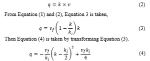
Based on the traffic theory, Greenshields equation is given by Equation (1).

v_f : free speed

k_j : jam traffic density

And the relationship between traffic volume (q) and traffic density (k) is provided by Equation (2) by traffic flow conservation law [8].

 

From Equation (1) and (4), the k – v curve and k – q curve are shown in Figure 1 (a) and (b).

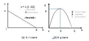
Figure 1: Fundamental Traffic Flow Curve

In terms of the traffic congestion from the traffic flow curve such as k – q curve, the traffic congestion area in the graph is shown in Figure 2.

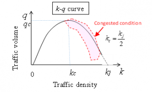
Figure 2: The traffic congestion area in k – q curve

The traffic congestion occurs after the critical traffic density (k_c) and eventually its traffic volume declines from this point. After reaching traffic jam density (k_j), the traffic volume becomes theoretically zero. In case of the k – v curve, the traffic congestion is located between k_c and kj as shown in Figure 3.

Figure 3. The traffic congestion are in k – v curve

2.2. Traffic Flow Measurement

In this research, the measurement field is used in Ahmedabad City of Gujarat State in India, where is one of big city in the state as mentioned in introduction. The traffic data is collected by 14 CCTV monitoring Cameras which are installed in the west side of the city as shown in Figure 4. In Figure 4, Camera#1 means CCTV number 1 and Camera#1 has one CCTV with pole on the street. The VMS#1 means VMS (Variable Message Sign board) number 1 and it also has CCTV with Traffic Sign board. The traffic data is measured by the CCTV and measures traffic flow data such as number of vehicles, average vehicles speed, traffic density. The traffic flow data was collected in June 2015 one month data by every minutes. The total traffic flow data for each CCTV becomes more than 40,000 points and author took 11 Camera data through Camera number 1 to 10 and VMS number. In this paper, we take eleven CCTV data because VMS#1 and VMS#2 data are missing during measurement by communication network error. In this traffic flow observation by traffic monitoring camera, we use major road traffic flow monitoring because the condition of intersection is different traffic flow with traffic signal and pedestrians. The intersection analysis is our next study.

Figure 4: Traffic monitoring Camera location in Ahmedabad city.

Among the result of measurement point, it takes the traffic flow data from Cameraera#2 in June 2015. The k – v curve and k – q curve are shown in Figure 5. Each data in Figure 5 shows generalized data by lane. In case of Cameraera#2 road, there are two lanes.

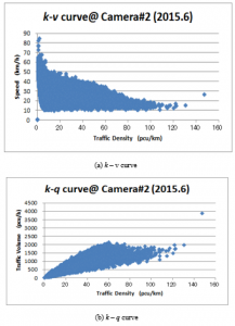
Figure 5: The measurement result of the traffic flow characteristics of Camera#2

From those two graphs, it is hard to define where traffic congestion point is.  Therefore, the daily traffic condition observation is shown in Figure 6 as daily basis traffic volume change and vehicle speed change from 7:00 am to 6:00 am next day.

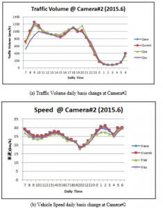
Figure 6: Traffic Flow Daily Basis Change at Camera#2

From Figure 6, it is clear that the evening time from 19:00 to 21:00 is most congested time zone because the vehicle speed is quite low (10km/h) than that of other time zone. But it is hard to know this condition from the traffic flow characteristics. In the next section, one of other traffic flow parameter is introduced to define traffic congestion condition.

3. Traffic Congestion Parameter

There are several traffic flow parameter such as occupancy, headway, and gap in the traffic monitoring data. Among those parameter, the occupancy is one of parameter which shows traffic condition. In this section, the occupancy parameter is described and it shows the relationship between occupancy and traffic volume. And after this, it is introduced new traffic congestion parameter “Traffic Congestion Triangle”.

3.1. Occupancy (OC)

The occupancy is one of traffic flow parameter to explain how vehicle is congested on the road how much vehicle occupies their road. From traffic flow theory, (OC) is defied by Equation (5).

where T is time of measurement, t_i is detected time of vehicle i.

When number of existing vehicles a certain section is N, average length of vehicle is , Equation (6) is given.

Therefore occupancy (OC) is proportional to traffic density (k) and traffic volume (q).

3.2. Relationship between Occupancy and Traffic Volume

From the one month measurement data of Camera #2 in June 2015, traffic volume (q) to occupancy (OC) relationship are shown in Figure 7. According to Figure 7, the relationship between (q) and (OC) is proportional and the number in the graph shows daily O’clock time such as 22 means 22:00. All the data is used from average from all time zone.

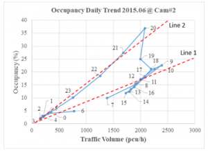
Figure 7: The Relationship between Traffic Volume and Occupancy at Camera#2

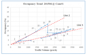
Figure 8: The Relationship between Traffic Volume and Occupancy at Camera#1

From Figure 7, there are two types’ lines which indicate the different growth ratio of the occupancy to the traffic volume. The Line 2 is large growth ration than that of the Line1 and the Line 2 starts from congested time zone from 20:00. The occupancy level

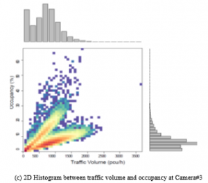
Figure 9: 2D Histogram between traffic volume and occupancy

is more than 30%, which means heavy congested condition as seen in Figure 6 (b). From this observation, there are two types of traffic congestion scenario like light traffic congestion by Line 1, which occurs normally in the morning and heavy traffic congestion by Line 2, which occurs normally in the evening. From our measurement records in June 2015, the traffic condition at Camera#2 is most congested than that of other locations. So, when it takes the case study of Camera#1, Figure 8 shows the relationship between the traffic volume to the occupancy. The occupancy value is lower than that of Camera #2, which means the traffic congestion at Cameraera#1 is smaller than at Cameraera#2.

3.3. “Traffic Congestion Triangle”

In the section 3.2, it takes the average value of each traffic volume and occupancy in June 2015 record. In case of the analysis from the total measurement, 2D histogram graph shows that of Camera#1, Camera#2, and Camera#3 in Figure 9. From Figure 9, each distribution of traffic volume and occupancy of Camera are different. In Camera#1 and Camera#3, it is clear two batches, which means there is clear traffic congestion condition between Line 1 and Line 2 in Figure 8 and Figure 10. On the other hand, there is not clear data batch between traffic volume and occupancy in Camera#2, which means Camera#2 area is relatively congested compared with Camera#1 and Camera#3. This is also able to explain by daily bases traffic volume and vehicle speed characteristics in Appendix Figure A. The vehicle speed of Camera #1 and Camera #3 is not so much drop during most congested time frame between 19:00 to 21:00.

As the observation of the relationship between the traffic volume and the occupancy, it is able to define the new traffic congestion parameter which illustrates as “Traffic Congestion Triangle” in Figure 10. The graph in Figure 10 is based on the measurement analysis at Camera #3. We have similar “Traffic Congestion Triangle” characteristics in other camera locations. Therefore this “Traffic Congestion Triangle” characteristics is common traffic flow characteristics in Ahmedabad city and it shows two types of traffic congestion trends in the morning and in the afternoon.

Figure 10: Traffic Congestion Triangle Concept

When we collect the traffic volume and the occupancy at each road in particular month, it is able to create the “Traffic Congestion Triangle” from the relationship between their average traffic volume and the occupancy daily basis. Then the “Traffic Congestion Triangle” line shows the occupancy growth ratio in daily basis traffic flow condition. According to our other observation analysis, we have similar trend of characteristics.

4. Conclusion

This study focuses the traffic congestion analysis in the developing countries, especially in India. And based on one month actual traffic data collection in one of typical major city of India―Ahmedabad―where its population is about 6 million, author creates new traffic congestion analysis parameter “Traffic Congestion Triangle”. This “Traffic Congestion Triangle” is able to indicate when and how the traffic congestion occurs in the city. And it shows there are two types of traffic congestion―high traffic destiny congestion( line1 in Figure 7,8) and low traffic density congestion (line2 in Figure 7,8). When we have this traffic congestion triangle at each road, it is easy to understand what kind of congestion occurs. However from this characteristics, it still does not provide solution how to reduce its traffic congestion. We only know its current condition.

We use one month data in June 2015 and the each item data becomes 43,200 (= 60 min use 10 traffic monitoring Cameras at main roads in the city and its traffic data is collected by very minute as traffic density, veh. × 24 hours × 30 days) points. After the detail traffic congestion observation, it is successful to show the unique relationship of traffic parameter between the traffic volume and occupancy. There are two patterns of occupancy growth ratio to the traffic volume in the morning and in the evening. According to all location traffic data analysis in Ahmedabad, the growth ratio in the evening is larger than that in the morning, which means its traffic congestion occurs in the evening time from 19:00 to 21:00. In the traffic volume to occupancy graph, those slope of two lines and the line between these two lines build the triangle shape, which it is defined as “Traffic Congestion Triangle” parameter. The members of “Traffic Congestion Triangle” indicates each traffic congestion condition. Therefore when the traffic volume and occupancy are detected, it is able to estimate how traffic congestion occurs and when its congestion goes to more crowded or smooth.

This study is based on June 2015 traffic data. So it is necessary to continue collecting and observing at all location such as whole year traffic data measurement. It is also necessary to check other major city case study at least in India and confirm that the “Traffic Congestion Triangle” is valid to other developing countries in future work.  It is also important to analyze the intersection point in terms of traffic congestion in future.

Conflict of Interest

The authors declare no conflict of interest.

Acknowledgment

This research is part of SATREPS program 2017 (ID: JPMJSA1606) between India and Japan.

1. Ahmedabad Municipal Corporation official website information: https://ahmedabadcity.gov.in/portal/jsp/Static_pages/demographics.jsp
2. Commissionerate of Transport Department of Port and Transport, Government of Gujrat data at http://rtogujarat.gov.in/statistics_vehicle.php
3. N. Gartner, C.J. Messer,A.K.Rathi, Traffic Flow Theory A State-of-the-Art Report: Committee on Traffic Flow Theory and Characteristics (AHB45), 2001.
4. C. Millikarjuna, K.R.Rao, Area occupancy characteristics of heterogeneous traffic, Journal Transportmetrica 2(3), 2006. Doi: https://doi.org/10.1080/18128600608685661
5. A. Salim, L. Vanajakshi, C. Subramanian, Estimation of Average Space Headway under Heterogeneous Traffic Conditions, International. of Recent Trends in Engineering and Technology, 3(5), 2010
6. M. Goutham and B. Chanda, Introduction to the selection of corridor and requirement, implementation of IHVS (Intelligent Vehicle Highway System) In Hyderabad, International Journal of Modern Engineering Research, 4(7), 49-54, 2014
7. B.D. Greenshields, A Study of Traffic Capaci, Proc.H.R.B., 14, 448-477, 1935.
8. W. Hole, 75 Years of Fundamental Diagram for Traffic Flow Theory Greenshields Symposium, Traffic Flow Theory Characteristics Committee, Transportation Research CIRCULAR, Number E-C149, 6, 2011.

(Click Here)

(Click Here)