1. Introduction

Servomotors have been developed at the origin of different uses. For example, radio-controlled aircraft, biped robots, and robotic arms. And nowadays, they are widely used in the robotics field, due to their cost, compactness, ease of use, and their high torque-to-weight ratio, which made them a good choice to achieve a compact and less expensive mechatronic system [1]. However, DCSM does not provide a good position control when it is in contact with a load and sometimes it provides a chattering motion. Thus, a mathematical model needs to be built to analyze and develop its performances. To do so, we tried to identify the mathematical equation of the system based on polynomial models.
A mathematical model is a multitude of equations that describe the relationship between the variables of a process or a phenomenon. It can take many forms depending on the studied system, and we can distinguish between two major classes.

1.1. Theoretical models

Theoretical models, Also known as whit-box, are models, which mostly used for simulations and theoretical studies. They are based on mathematical and physical laws, which made them often complex and hard to define [2]; however, it can give a complete description of the system.

1.2. Experimental models

Experimental models, also known as grey-box or black-box models are models used to define a mathematical model from the experiment’s data. As mentioned in [3], in system identification, we could distinguish between two types.
non-parametrical model is usually presented with numerical values, a graph, or a table, and it has an infinite number of parameters and an undefined structure.
parametrical models, which are defined models structure who have a finite number of parameters.
According to [4], identifying a system or a process is about estimating a mathematical model that reproduces a static and dynamic response to a test input as close as possible to the real system. To do so, and to get a valid model, we need to follow a certain procedure [5], described in fig.1. It starts with the experiment preparation by choosing the sampling frequency and the input signal as a first step. Then choosing the model structure type, order, and delay as a second step. After that, selects the criterion that minimizes the error between the estimated model and the experimental data as the third step. Finally, the validation step that consists of applying several tests to prove the usability of the model. The resulting models’ main objectives can be to understand the behavior of the studied system [6], or building the system control loop [7].
In this paper, Sections 2 and 3 cover a brief introduction of the linear polynomial models and parameter estimation process. Section 4 and 5 highlight the necessary steps for the implementation of the application. In sections 6 and 7, the results obtained from the experiment are presented and discussed.

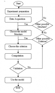
Figure 1: Experimental approach for defining a parametric model of a system

Figure 2: Generalized transfer function Structure

2. Parametrical Models

2.1. Generalities

A discrete linear system can be presented as a general-linear polynomial model, which is considered as a transfer function whose parameters need to be estimated. This estimation is done by recursive and none recursive algorithms like maximum likelihood, instrumental variable or less square. This presentation, also gives flexibility for modelling both stochastic and system dynamics, and it is widely used in many real-world applications from different disciplines, e.g., [8–10].
Polynomial models are described in [11]. They can be defined by the generalized transfer function expressed by (1) and the signal flow represented in figure 2 [5]:

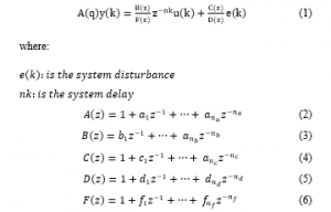
and:
n_a : The order of A(z)
n_b : The order of B(z)
n_c : The order of C(z)
n_d : The order of D(z)
n_f : The order of F(z)
By setting one or more n_a, n_c,n_d and n_f to 0 can create simpler models such as:

2.1.1. ARX model

ARX structure presented in equation (7) [5] is the result of setting n_c,n_d and n_f to 0 the signal flow is presented in fig.3. In this structure the noise model 1/A(z) is coupled with the systems dynamics, it is used to obtain simple model with good signal to noise ratio.

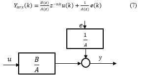
Figure 3: The ARX Structure

2.1.2. ARMAX model

The ARMAX structure presented in the equation (8) [5] is the result of setting n_d and n_f to 0 in the generalized transfer function (1), the signal flow is presented in fig.4. this structure provides more flexibility to model the noise by adding the C(z) parameters which is considered as a moving average of white noise. It is used when the noise enters in the input.

Figure 4: The ARX Structure

2.1.3. Output Error Model

The OE presented in the equation (9) [5] is the result of setting n_a, n_c and n_d to 0 in the generalized transfer function (1), the signal flow is presented in fig.5. In this structure, the noise model is considered as 1. It is used to parameterize the dynamic of the system only.

Figure 5: The OE Structure

 

2.1.4. Box- Jenkins Model

The BJ structure presented in the equation (10) [5] is the result of setting n_d to 0 the signal flow is presented fig.6. This structure provides more flexibility because the noise model is independent of the dynamics model. It is used when the noise enters as a measurement disturbance.

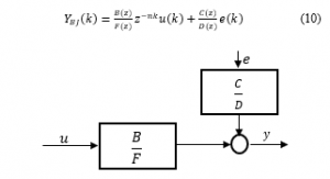
Figure 6: The BJ Structure

 

3. Parameters Estimation

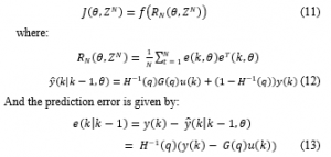
Parameter estimation is a mathematical process that uses experimental data to estimate the system parameters, in this paper; this process is done by the prediction error method described in [12] and fig 7. this method aims to minimize the error expressed in Eq (13) between the estimated and the real system [13].

Figure 7: Prediction Error Method

According to [14], to use the Prediction Error Method, we need to choose the model structure, the one-step-ahead predictor y ̂(k│k-1,θ) described with the equation (12) and the criterion function J(θ,Z^N ) given by Eq (11):

4. Model Validation

Model validation is the final step, which goal is to compare and validate the usability of the estimated model by testing several criterions like those in this paper:
Akaike Final Prediction Error
This criterion described in the equation (14) [5] was presented by Akaike (1967) as a final prediction error (FPE), based on Akaike’s theory, the best model has the smallest FPE.

where:
N: The number of values in the estimation data set
e(t): The vector of prediction error
θ_N: The estimated parameters
d: The number of the estimated parameters

4.1. Best Fit

The RMSE criterion measures the similarity between the data and the estimated model and can be calculated using equation (15) [15].

where:
y_i : The measured output
y ̂ : The estimated output
y ̅: The mean of the output

5. Application

A DCSM is composed of a potentiometer and integrated circuit that ensures a dc motor’s position control based on a reference signal received from a microcontroller or an external organ (fig.8). However, despite its different applications, there is a major problem in achieving good performance with those servo motors due to the integrated circuit [1]. Therefore, the goal is to estimate all the system’s internal and external components’ mathematical model, to design a new controller or exploit it in more complex systems. In this application, the reference signal is in the form of a pulse with modulation signal who does not exceed 20ms between two rising edges, and the DCSM supply voltage is 5V.

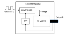
Figure 8: Internal structure of a DC Servomotor

Figure 9: Data acquisition board schema

To extract reliable input and output data, we build the acquisition card with pic16f877a. As shown in fig 9, this microcontroller has eight analogic inputs of 10-bit resolution, one digital input, one digital output of 8-bit resolution, and two PWM output of 8-bit resolution. Moreover, it is linked to the computer using RS232 communication with a speed of 115200bit/s to send and receive data necessary for the experiment. However, today’s computer does not support this type of communication. To solve this problem, an RS232 to USB adapter is used, as shown in fig 10.

Figure 10: Typical block diagram of the experiment

Afterward, to know the sampling time Ts, which is related to the uncertainty of the internal and external components and the instructions execution time of the microcontroller. The analogic input of the acquisition card is subjected to a periodic signal of known frequency. The samples collected from the acquisition card are represented on a graph. Afterward, the frequency of the test signal is adjusted until a signal similar to that of the input is obtained, which Ts = 0.0034 deduced in this application. This will allow having a speed of 300 sps/s.
Next, the analysis and parameter estimation process is applied to the collected data from the acquisition card.

6. Results

Model order determination in parameter estimation is essential because a lower order model cannot adequately describe the system’s dynamics, and a higher-order model may have uncertainties. Thus, to extract the best model and to see the effect of changing the order of the parameters, we applied the experimental approach of identifying a parametric model described in fig 1, and we fixed nk to 1 then:
Over 100 ARX models are calculated where n_aand n_b are in the range of 1 to 10.
Over 125 ARMAX models are calculated where n_a,n_b and n_c are in the range of 1 to 5.
Over 25 OE models are calculated where n_f 〖and n〗_bare in the range of 1 to 5.
Over 625 BJ models are calculated where n_a,n_a,n_a and n_a are in the range of 1 to 5.
Afterward, the Best-fit criterion is used to select the best five structures in each model, and the PFE criterion is used to choose the best structure in each model. Those results are in tables 1 to 4.

7. Discussion

As presented in tables 1 to 4, all the extracted models in each structure have closely a similar FPE. Then the choice of the model is based on the best-fit only. Besides, no significant change occurs in the best-fit criterion by increasing the models’ order in each model type. Thus, the selected model will have the lowest order. This will allow a better processing time while doing online parameter estimation in real-time applications.
The best-estimated ARX model is the ARX331 shown in Figure 11 and Table 1. It has an order of (nb=3 and na = 3), and a fit of 72,44
The best-estimated ARMAX model is the ARMAX2411 shown in Figure 12 and Table 2. It has an order of (na = 2, nb = 4, nc=1), and a fit of 94,75%.
The best-estimated OE model is the OE131 shown in Figure 13 and Table 3. It has an order of (nf = 3, nb = 1), and a fit of 95.009.
The best-estimated BJ model is the BJ12331, shown in Figure 14 and Table 4. It has an order of (nb = 1, nc = 2, nd = 3, nf = 3), and a 95.02% fit.
Based on those results and figure 16. The ARX models provided a fit of 72%, which is a poor fit compared to ARMAX, BJ and OE Models. However, if we want to use a model in real-time applications, the best choice will be OE131 because of the resulting good fit with the measured output and fewer parameters.
Table 1: The estimated ARX models

Model Type	Model Parameters	‘Best Fit’	‘FPE’
‘ARX431’	A(z) = 1 – 1.065 z^-1 + 0.005417 z^-2 + 0.01607 z^-3 + 0.04765 z^-4 B(z) = 3.841e-05 z^-1 + 0.002391 z^-2 + 0.001677 z^-3	72,6272093	0,3764651
‘ARX441’	A(z) = 1 – 1.065 z^-1 + 0.005351 z^-2 + 0.01617 z^-3 + 0.04766 z^-4 B(z) = 3.741e-05 z^-1 + 0.002391 z^-2 + 0.002752 z^-3 – 0.001086 z^-4	72,5563214	0,37670021
‘ARX421’	A(z) = 1 – 1.065 z^-1 + 0.005566 z^-2 + 0.01616 z^-3 + 0.04759 z^-4 B(z) = 3.772e-05 z^-1 + 0.004052 z^-2	72,5177552	0,37624736
‘ARX331’	A(z) = 1 – 1.069 z^-1 + 0.005651 z^-2 + 0.06704 z^-3 B(z) = 0.000315 z^-1 + 0.002366 z^-2 + 0.001609 z^-3	72,4480688	0,37718277
‘ARX341’	A(z) = 1 – 1.068 z^-1 + 0.005065 z^-2 + 0.06748 z^-3 B(z) = 0.0003129 z^-1 + 0.002366 z^-2 + 0.002673 z^-3 – 0.001074 z^-4	72,386256	0,37731582

Table 2: The estimated ARMAX models

‘Model Type’	Model Parameters	‘Best Fit’	‘FPE’
‘ARMAX3421’	A(z) = 1 – 2.598 z^-1 + 2.202 z^-2 – 0.6041 z^-3 B(z) = 0.001024 z^-1 + 0.002355 z^-2 – 0.008141 z^-3 + 0.004814 z^-4 C(z) = 1 – 1.576 z^-1 + 0.5755 z^-2	94,8596855	0,36096562
‘ARMAX2421’	A(z) = 1 – 1.985 z^-1 + 0.9851 z^-2 B(z) = 0.001351 z^-1 + 0.0005912 z^-2 – 0.006229 z^-3 + 0.004419 z^-4 C(z) = 1 – 0.9752 z^-1 – 0.02485 z^-2	94,7854814	0,36124302
‘ARMAX4231’	A(z) = 1 – 2.362 z^-1 + 1.557 z^-2 – 0.02015 z^-3 – 0.1743 z^-4 B(z) = -0.0004067 z^-1 + 0.0004638 z^-2 C(z) = 1 – 1.312 z^-1 + 0.1561 z^-2 + 0.156 z^-3	94,7787217	0,36258016
‘ARMAX2411’	A(z) = 1 – 1.986 z^-1 + 0.9859 z^-2 B(z) = 0.001361 z^-1 + 0.0006902 z^-2 – 0.006188 z^-3 + 0.004261 z^-4 C(z) = 1 – z^-1	94,7591717	0,3611956
‘ARMAX3411’	A(z) = 1 – 2.022 z^-1 + 1.059 z^-2 – 0.03639 z^-3 B(z) = 0.001229 z^-1 + 0.0009276 z^-2 – 0.00656 z^-3 + 0.004529 z^-4 C(z) = 1 – z^-1	94,7457863	0,36131993

 

Table 3: The estimated OE models

‘Model Type’	Model Parameters	‘Best Fit’	‘FPE’
‘OE431’	B(z) = 0.01849 z^-1 – 0.05449 z^-2 + 0.05356 z^-3 – 0.01755 z^-4 F(z) = 1 – 2.947 z^-1 + 2.894 z^-2 – 0.9475 z^-3	95,0341979	6,13354962
‘OE131’	B(z) = 7.423e-06 z^-1 F(z) = 1 – 2.933 z^-1 + 2.867 z^-2 – 0.9339 z^-3	95,0098583	6,28005407
‘OE341’	B(z) = 0.01923 z^-1 – 0.03923 z^-2 + 0.02007 z^-3 F(z) = 1 – 2.14 z^-1 + 0.8912 z^-2 + 0.6443 z^-3 – 0.3956 z^-4	94,9929819	6,21730334
‘OE321’	B(z) = 0.04349 z^-1 – 0.08893 z^-2 + 0.04559 z^-3 F(z) = 1 – 1.984 z^-1 + 0.9845 z^-2	94,9848311	6,21616865
‘OE221’	B(z) = -0.001383 z^-1 + 0.001513 z^-2 F(z) = 1 – 1.985 z^-1 + 0.9851 z^-2	94,8945691	6,55918215

 

Table 4: The estimated BJ models

‘Model Type’	Model Parameters	‘Best Fit’	‘FPE’
‘BJ23241’	B(z) = 6.176e-05 z^-1 – 5.46e-05 z^-2 C(z) = 1 – 0.6253 z^-1 + 0.01001 z^-2 + 0.02315 z^-3 D(z) = 1 – 1.629 z^-1 + 0.6427 z^-2 F(z) = 1 – 2.44 z^-1 + 1.393 z^-2 + 0.5362 z^-3 – 0.4889 z^-4	95,0238364	0,360708
‘BJ12331’	B(z) = 7.101e-06 z^-1 C(z) = 1 – 1.609 z^-1 + 0.9796 z^-2 D(z) = 1 – 2.46 z^-1 + 2.254 z^-2 – 0.7828 z^-3 F(z) = 1 – 2.936 z^-1 + 2.872 z^-2 – 0.9367 z^-3	95,0160798	0,33251152
‘BJ14131’	B(z) = 7.24e-06 z^-1 C(z) = 1 + 0.04146 z^-1 + 0.03341 z^-2 + 0.01694 z^-3 + 0.03648 z^-4 D(z) = 1 – 0.9637 z^-1 F(z) = 1 – 2.934 z^-1 + 2.87 z^-2 – 0.9354 z^-3	95,0135709	0,36037501
‘BJ13131’	B(z) = 7.263e-06 z^-1 C(z) = 1 + 0.04056 z^-1 + 0.03335 z^-2 + 0.01701 z^-3 D(z) = 1 – 0.9659 z^-1 F(z) = 1 – 2.934 z^-1 + 2.869 z^-2 – 0.9351 z^-3	95,0131615	0,36038438
‘BJ13231’	B(z) = 7.26e-06 z^-1 C(z) = 1 – 0.6241 z^-1 + 0.009762 z^-2 + 0.02454 z^-3 D(z) = 1 – 1.627 z^-1 + 0.6415 z^-2 F(z) = 1 – 2.934 z^-1 + 2.87 z^-2 – 0.9353 z^-3	95,0129791	0,35994338

 

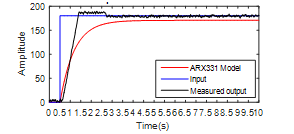
Figure 11: Comparison between the estimated model (ARX331) and measured output

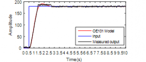
Figure 12: Comparison between the estimated model (OE131) and measured output

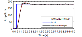
Figure 13: Comparison between the estimated model (ARMAX2411) and measured output

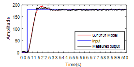
Figure 14: Comparison between the estimated model (BJ1313) and measured output

Figure 15: Comparison between the estimated Polynomial models (ARX331, ARMAX2411, OE131, and BJ1313) and measured output

8. Conclusion

In this article, a practical identification of DCSM has been elaborated using polynomial models. To meet application requirements and to collect input-output data, a microcontroller-based acquisition card has been developed. Finally, the comparison between the data and the estimated models using validation criterions shows that the ARMAX, BJ, and OE model has provided a good fit with experimental data and can be used in simulations or a real application.
In future work, the data acquisition system will be based on PLC to be adequate for industrial applications and to provide more sampling frequency and processing time. Moreover, other identification techniques will be applied to more complex non-linear systems to build proper algorithms for the control loop or fault detection.

1. T. Wada, M. Ishikawa, R. Kitayoshi, I. Maruta, T. Sugie, “Practical modeling and system identification of R/C servo motors,” in 2009 {IEEE} International Conference on Control Applications, IEEE, 2009, doi:10.1109/cca.2009.5280987.
2. L. Ljung, “Perspectives on system identification,” Annual Reviews in Control, 34(1), 1–12, 2010, doi:10.1016/j.arcontrol.2009.12.001.
3. R. Isermann, M. Münchhof, Identification of dynamic systems: an introduction with applications, Springer Science & Business Media, 2010.
4. M. Villain, Systèmes asservis linéaires, Ellipses, 1996.
5. L. Lennart, “System identification: theory for the user,” PTR Prentice Hall, Upper Saddle River, NJ, 1–14, 1999.
6. M. Jirgl, L. Obsilova, J. Boril, R. Jalovecky, “Parameter identification for pilot behaviour model using the {MATLAB} system identification toolbox,” in 2017 International Conference on Military Technologies ({ICMT}), IEEE, 2017, doi:10.1109/miltechs.2017.7988824.
7. S. Rai, S.-Y. Yang, T.-C. Tsao, “Wind turbine system identification and individual pitch control,” in 2017 American Control Conference ({ACC}), IEEE, 2017, doi:10.23919/acc.2017.7963144.
8. S. Rachad, B. Nsiri, B. Bensassi, “System Identification of Inventory System Using {ARX} and {ARMAX} Models,” International Journal of Control and Automation, 8(12), 283–294, 2015, doi:10.14257/ijca.2015.8.12.26.
9. W. Araydah, T.A. Tutunji, I. Al-Naimi, “System identification for a liquid flow process,” in 2017 {IEEE} Jordan Conference on Applied Electrical Engineering and Computing Technologies ({AEECT}), IEEE, 2017, doi:10.1109/aeect.2017.8257756.
10. S.L. Chavan, D.B. Talange, “System identification black box approach for modeling performance of {PEM} fuel cell,” Journal of Energy Storage, 18, 327–332, 2018, doi:10.1016/j.est.2018.05.014.
11. L. Ljung, “Black-box models from input-output measurements,” in {IMTC} 2001. Proceedings of the 18th {IEEE} Instrumentation and Measurement Technology Conference. Rediscovering Measurement in the Age of Informatics (Cat. No.01CH 37188), IEEE, 2001, doi:10.1109/imtc.2001.928802.
12. L. Ljung, “Prediction error estimation methods,” Circuits, Systems, and Signal Processing, 21(1), 11–21, 2002, doi:10.1007/bf01211648.
13. M. Brunot, A. Janot, F. Carrillo, M. Gautier, “A Separable Prediction Error Method for Robot Identification,” {IFAC}-{PapersOnLine}, 49(21), 487–492, 2016, doi:10.1016/j.ifacol.2016.10.650.
14. Y. Zhao, B. Huang, H. Su, J. Chu, “Prediction error method for identification of {LPV} models,” Journal of Process Control, 22(1), 180–193, 2012, doi:10.1016/j.jprocont.2011.09.004.
15. L. Ljung, System identification toolbox. Getting started guide. The Mathworks Inc, 2017.

(Click Here)

(Click Here)