1. Introduction

Recognizing facial emotions is a challenging and interesting task, proven with numerous previously held competitions [1–8], available datasets [1, 9–14], and conducted researches on the subject. The progresses made for computer vision in recognizing emotion by face have been described in many publications [15–19]. A notable mention is the extensive paper by Li and Deng [19] which gives explanatory and thorough review about existing and commonly used datasets for facial emotion recognition, along with state-of-the-art (SOTA) approaches and their respective results.

The reviews from [15–19] described many available facial emotion recognition datasets, such as Facial Emotion Recognition 2013 (FER-2013) [1, 9], Static Facial Emotion in the Wild (SFEW) [10], Japanese Association of Female Facial Expression (JAFFE) [11], Cohn-Kanade (CK) [12], Extended Cohn-Kanade (CK+) [13], and Expression in the Wild (ExpW) [14] among many others. These datasets vary in many aspects, commonly described by one or combination of the following: amount of data, number of emotion classes, image- or sequential-based, and in lab-like or in-the-wild condition. The amount of data available in each dataset varies from hundreds to tens of thousands, with some datasets having pre-set training, validation, and/or testing data distribution. These datasets also vary in number of emotion classes, commonly ranging from six to eight emotion classes which include anger, disgust, fear, happiness, sadness, surprise, contempt, and is often appended with neutral emotion as well. Although some datasets do not include neutral and/or contempt expression. Image- or sequential-based (video-based or image-sequence-based) datasets also give variance in the conducted researches, as each dataset type’s processing require different approach. Another difference is the condition of the dataset, where lab-like dataset differ from in-the-wild dataset. The former is recorded in an ideal condition (proper lighting, proper face alignment, and/or minimal to no usages of face accessories such as eyeglasses), whereas the latter depicts face expressions captured in a non-ideal condition from real-world scenarios.

These datasets are utilized in many works related to solving facial emotion recognition task, some of which uses conventional methods, deep learning, pretrained model, ensemble neural networks, combination of deep learning with hand-crafted feature selection technique(s), and other related works that will be described in following sections. These approaches achieve various results, which could be summarized in most researches’ test accuracy for lab-like datasets often achieving above 90%, while test accuracy for in-the-wild datasets barely surpasses 75% [19].

With such low accuracy result from previous researches for facial emotion recognition with in-the-wild dataset (as compared with lab-like datasets), this paper attempts to improve facial emotion recognition accuracy for image-based in-the-wild dataset FER-2013. The proposed model achieved test accuracy of 69.40%, which is better than most existing researches with standalone-based neural network architecture, with the advantage of being simpler in terms of network depth and topology and having the capability of end-to-end training.

Continuing this introduction is a review of core concepts, brief description of FER-2013 as the used dataset in this paper’s experiments, existing approaches for facial emotion recognition task using FER-2013 dataset, and the works that inspire and are the base of this paper’s model. Afterwards, the proposed model is elaborated in detail. Then, the results from the proposed model are discussed and compared with other related works to understand how well the model performs compared to other taken approaches. Finally, this paper concludes with final thoughts about the proposed model and future works to improve facial emotion recognition task.

2. Literature Review

2.1. Studies and Developments

The study of emotion has gained interest since early 1970s, with one remarkable and frequently used research result being the work of Ekman and Friesen. They introduced six basic emotions: anger, disgust, fear, happiness, sadness, and surprise [20]. Many publications would later improve the known basic emotions, such as the work of Matsumoto which described contempt as another universal basic emotion [21]. Other improvements include the introduction of tools for supporting study of emotion recognition, such as the development of Facial Action Coding System (FACS) [22] with the updated version introduced in 2002 [23].

The interest in emotion study gained attention from computer science researchers as well, resulting in published researches on how to create automated emotion recognition system since the late 1980s. Even a survey on the developments made during those times [24]. These researches were conducted with broad and separate focus, such as establishing dataset [11, 12, 25], mapping features or feature selection process(es) [26, 27], designing architecture [27, 28], and adopting approaches from other fields of study [25, 27]. More recent studies adopted CNN for face emotion recognition, such as the approaches proposed in [29–31]

One, if not the most, attractive feature of emotion recognition is the human face itself. The main reason behind this is because mostly human face expresses emotions one feels [32]. The expression(s) is/are shown due to the work of face muscles’ coordination which produces many expression configurations [33]. Note that the human face can express more than one emotion at the same time or at an approximately same time [34].

2.2. Facial Emotion Recognition Dataset (FER-2013)

For such an attractive feature, many datasets have been developed for facial emotion recognition task. As this paper only utilizes one dataset (FER-2013 [1,9]), it is the only dataset discussed in the paper.

Created in 2013, FER-2013 dataset contains 35,887 grayscale 48×48-pixel images, with the images being stored in a spreadsheet where each image’s pixel values are stored in cells per row. The images were obtained utilizing Google search and are later grouped per emotion classes, which are anger, disgust, fear, happiness, neutral, sadness, and surprise. As the dataset was built utilizing Google search, the images are in in-the-wild condition, with even very few images being animated characters.

The dataset originally had data distribution of 28,709 images for training and 3,589 images for public test, but after the competition ended, another 3,589 images which were used for private test were added to the dataset. The usages of FER-2013’s data distribution vary among published researches, with each using public test images for different purposes, either as part of training set, validation set, or test set. Several images contained in FER-2013 dataset are given in Figure 1.

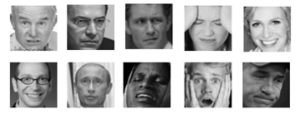
Figure 1: FER-2013 sample images

2.3. Standalone-Based Neural Network (SBNN)

An architecture was proposed using CNN and batch normalization, in which the batch size was set constant to 256. The training process ran for 8 epochs as higher epochs was reported to result in overfitting [35]. Such architecture resulted in 60.12% test accuracy on FER-2013’s private test data.

Other architectures using both CNN and batch normalization, varying in number of filters, were proposed in [36]. The uniqueness of both architectures is that both do not have any fully connected layer and maintain kernel size of 8, and with this design, both architectures achieved test accuracy above 65%.

Global average pooling (GAP) [37] was also used as an addition to both CNN and batch normalization [38]. The architectures vary in terms of depth-wise separable convolution layer, and although both were designed for multi-task purposes (emotion and gender recognition), both architectures achieved 66% accuracy.

Another new architecture inspired by network-in-network architecture and Inception was proposed with addition of utilizing a polynomial-based learning rate decreasing method for faster convergence and better performance [39]. The data used as input were pre-processed first for face feature extraction while still maintaining the image form, which resulted in a maximum of 10% increase in accuracy. With the proposed architecture and data pre-processing, the test result for FER-2013 dataset reached 66.4% after training for 200 epochs with batch size of 250, noting that the test data used is unknown to be either public or private test data.

Two SBNN architectures, one using custom CNN and another using One-vs-All (OVA) Support Vector Machine (SVM) with Histogram of Oriented Gradients (HOG) which resulted in 66.67% and 45.95% accuracy on test data of FER-2013 dataset respectively were also introduced [40].

A new SBNN architecture based on attentional convolutional neural networks was proposed in [41]. The proposed model was able to focus on only face features that are important to emotion recognition, achieving 70.02% test accuracy on FER-2013’s private test data.

The winner of FER-2013 challenge, Yichuan Tang, proposed SBNN architecture with L2-SVMs (DLSVM) as replacement for softmax layer at the end of the neural network architecture. Such modification resulted in the proposed model reaching 71.2% test accuracy on private test dataset [42].

The current SOTA SBNN architecture was proposed in [43], in which they theorized that features at mid-level and high-level of a CNN would have impact on the final prediction. They based their model, termed as Multi-Level Convolutional Neural Network (MLCNN), on VGG architecture with 18 layers and achieved 73.03% test accuracy on FER-2013’s private test data.

2.4. Ensemble-Based Neural Network (EBNN)

An EBNN architecture with 3 subnets, containing 3 and increasing convolution layers respectively for each subnet was proposed [44]. With batch size of 100, momentum value of 0.9, learning rate value of 0.01 decreasing to 0.001 by validation error condition, and running from varying epochs of 20 to 100, and 80% and 20% data distribution for training and test set respectively, they reached 65.03% test accuracy.

Referred in their paper as aggregator or hybrid CNN–SIFT aggregator, [45] combined CNN with Scale Invariant Feature Transform (SIFT), specifically Dense SIFT and regular SIFT. The EBNN, constructed and trained from scratch with combining CNN, Dense SIFT, and regular SIFT, resulted in 73.4% test accuracy on FER-2013 private test data.

Another researcher proposed an EBNN coined as hierarchical committee for facial emotion recognition task with 216 retrained deep convolutional neural network (DCN) models using transfer learning and 108 DCN models trained on aligned faces [46]. This method achieved 70.58% test accuracy on FER-2013’s private test dataset, with randomly splitting training data for training and validation purposes after removing 11 images from the training data. The work is further developed in [47] which consisted of 9 DCNs, with each having 3 convolution-max pooling stages and ended with 2 fully connected layers. By using both aligned and non-aligned face structure dataset in training each DCN and using Alignment-Mapping Network (AMN) with the ensemble, they achieved 73.73% accuracy on FER-2013 private test data with the same training and validation data distribution as used in [46].

Another proposed EBNN architecture was offered in Pramerdorfer and Kampel’s work [48]. The ensemble consisted of 8 DCN models based on VGG, Inception, and ResNet, where each base model underwent convolution and/or pooling layer(s) removal. They managed to achieve 75.2% test accuracy on FER-2013 private test data.

Currently known SOTA EBNN architecture was proposed in [49], which combined 3 VGG models, 2 pre-trained models which were retrained, and 1 model trained from scratch, combined with SIFT and k-means clustering, and flattened extracted feature vector as input to local SVM. This approach achieved 75.42% test accuracy on FER-2013’s private test data.

2.5. Other Researches

There are other notable researches that inspire the proposed model which impacts the proposed model’s architecture and learning and/or generalization capability. These researches are reviewed in this section in the order of previously stated impact descriptions, with the purpose of giving brief and proper information regarding the researches’ results prior to elaborating the proposed model.

The architecture of the model is based on VGG-16 architecture [50], which contains 13 convolution layers with 3 additional fully connected layers at the end of the network. After each convolution layer, ReLU [51] layer is used for non-linearity rectification. Table 1 describes VGG-16 architecture.

Table 1: VGG-16 architecture

Type	Layer
Feature Extractor	Convolution
	Convolution
	Max Pooling
	Convolution
	Convolution
	Max Pooling
	Convolution
	Convolution
	Convolution
	Max Pooling
	Convolution
	Convolution
	Convolution
	Max Pooling
	Convolution
	Convolution
	Convolution
	Max Pooling
Classifier	Dense/Fully Connected (4096)
	Dense/Fully Connected (4096)
	Dense/Fully Connected (1000)
	Softmax

However, the existence of fully connected layers in a convolutional neural network architecture may lead to higher overfitting probability [37]. To overcome this, the authors in [37] proposed GAP which works by averaging each of final feature map results and directly using the averaged results for classification. This pooling method regularizes feature maps as confidence map for categories with no parameter requiring optimization, hence avoids overfitting.

Another attempt to reduce overfitting possibility is the use of early stopping [52]. Such implementation affects the training mechanism as the training may stop before fully reaching the specified number of epochs due to no further increase in accuracy or decrease in loss in a specific period. Other than using early stopping to avoid overfitting, a proper optimizer is required for better model learning and/or generalization capability.

One most used and popular optimizer is Stochastic Gradient Descent (SGD) [53, 54], which takes constant parameter learning rate and traverses the gradient by the specified learning rate to find global minima. With SGD, it was reported that the generalization capability of a model improves [55, 56], hence less overfitting probability. Another development for SGD was using momentum as additional parameter which accelerates model learning process, which has been proven in practice in [57]. However, SGD is often slow for learning process since the traversing process is done uniformly by the learning rate value.

An alternative to SGD was proposed in [58] and coined as Adam to overcome SGD’s limitation. With Adam, the learning process adapts the learning rate parameter as the learning process continues, resulting in better learning performance compared to SGD. The major drawback of Adam is the generalization capability drops significantly as reported in [56].

      In an effort to overcome Adam optimizer’s drawback, Keskar and Socher proposed SWATS (Switching from Adam to SGD) [59], which at first uses Adam optimizer to have better initial learning process then switches to SGD on specified trigger condition. They empirically argued that SWATS optimizer gives better performance on most tasks, especially visual- and text-based tasks, by combining both Adam and SGD.

3. Proposed Model

Our proposed model was defined to be based on VGG-16 as the base model and using GAP as final pooling layer prior to VGG-16’s classifier. The best model was obtained after experimenting on multiple combinations of SGD/Adam/SWATS as optimizer and inclusion/non-inclusion of early stopping. The researchers made some modifications for VGG-16’s classifier due to the use of GAP.

VGG-16 was chosen as the base model for several reasons. The first reason is because VGG-16 uses convolution layer with 3×3 kernel instead of 5×5 or 7×7, hence lesser parameters to train [50]. The second reason is by using two or three stacked convolution layers with 3×3 kernel as an equal for one convolution layer with 5×5 or 7×7 kernel respectively, VGG-16’s architecture adds more rectification layers, which results in a decision function that is more discriminative [50]. The third reason is based on empirical findings as the researchers reviewed previous publications, in which the researchers found that several SBNN and EBNN researches used VGG based models and achieved good, with some achieving SOTA, results on FER-2013 dataset among other tested datasets. While VGG-13, VGG-16, and VGG-19, either in its original architecture or modified, are present in the found literature reviews, the researchers decided to go with VGG-16 since it is not too deep and complex as VGG-19, noting that both architecture demonstrated similar results as reported in [50]. The researchers also agreed to not use VGG-13 as Simonyan and Zisserman stated in their paper that increase in depth in networks results in better accuracy [50]. In addition to the architecture selection, the researchers theorized that the use of pretrained model may improve accuracy and reduce training time. The researchers used VGG-16’s pretrained model which was trained on ImageNet [60] dataset rather than initializing the network’s weights randomly.

The researchers also modified VGG-16’s architecture by using GAP as final pooling layer before entering VGG-16’s classifier, and therefore the researchers replaced all of VGG-16’s classifier layers with a single fully connected layer, taking 512 averaged input neurons and outputting 7 neurons as the equivalent number of FER-2013’s emotion classes. Our proposed model’s architecture can be seen in Table 2.

With the proposed model’s architecture, the researchers experimented on multiple combinations of training mechanism, optimizer choices, data distribution, frozen layers, and batch normalization usage. Our best model was trained using SGD optimizer and used early stopping in its training process. Such combination proved to be superior as compared with the researchers other experiments. The results of the experiments are discussed in the next section.

Table 2: Modified VGG-16 architecture

Type	Layer
Feature Extractor	Convolution
	Convolution
	Max Pooling
	Convolution
	Convolution
	Max Pooling
	Convolution
	Convolution
	Convolution
	Max Pooling
	Convolution
	Convolution
	Convolution
	Max Pooling
	Convolution
	Convolution
	Convolution
	Global Average Pooling
Classifier	Dense/Fully Connected (7)

4. Experiments

4.1. Experimental Design

The researchers experimented on combining VGG-16 with several optimizers and training method. The used optimizers were SGD, Adam, and SWATS, and the training method was customized to use early stopping. The experiment was conducted using PyTorch and ran on Google Colab with GPU acceleration support. Due to the training data’s size and Google Colab’s lifetime, the researchers had to perform run-and-pause per 10 epochs as part of the training mechanism to prevent sudden disconnect from the machine, since in such an event the training process may stop prematurely. Note that the training and validation were done in one epoch. After each run-and-pause, the test was performed per 10 epochs on the model and the results are recorded.

Initially, the researchers had several options to experiment on. The options include the use/disuse of batch normalization, freezing/not freezing selected layers, imbalanced (original)/balanced training data distribution, use/disuse of GAP, and SGD/Adam/SWATS optimizer selection. All in all, the researchers initially estimated the need to experiment on approximately 12 combinations of VGG-16 model. Due to the quite large number of possible combinations and since each epoch takes about 7-10 minutes, the researchers had to estimate which combination merits further investigation per specified run epochs. After each combination has passed the specified run epochs, the combination that provided the highest test accuracy was used to undergo further training and/or further combination. At the end of the experiments, the researchers experimented on 23 combinations, with all combinations having equivalent hyperparameter values. The researchers used learning rate value of 0.001, 0.9 for momentum on SGD optimizer, and batch size of 32.

The results of the experiments are given in Table 3. For better readability, the following acronyms are used in Table 3:

• EG: Experiment group

The researchers group the experiments to select the best model in each experiment group, and what the next experiment group’s models’ possible combinations are.

• D: Data distribution

FER-2013 dataset is very imbalanced, with some classes having more than 5,000 images and some having less than 1,000 images. The researchers tried using both balanced and imbalanced FER-2013 dataset to see which would yield better results. The acronyms for the experiments’ FER-2013 data distribution are as follows:

• B: Balanced
• I: Imbalanced

• BN: Use batch normalization

The use of batch normalization should help the model learn in a more stable manner, yet some of the best performing SBNN models do not use batch normalization. To this extent the researchers included the combination of using and discarding batch normalization in the model.

• GAP: Use global average pooling (GAP)

GAP layer helps aggregate feature map information and helps prevent overfitting caused by fully connected layers in the model. For this reason, the researchers tried the combination of using and not using GAP in the experiments. Note that although GAP can be used as the classifying layer, the researchers appended a fully connected layer instead as the classifying layer for GAP’s aggregated feature map.

• LL: Learning layers

Finetuning a pretrained model can be done with freezing some layers except for the new classifier layer(s). Our experiments freeze some layers and keep others to be able to learn (learning layers). The following acronyms show possible combinations of learning layers in the experiments:

• F447: Fully connected layers with neurons structure 4096-4096-7
• F7: Fully connected layer with 7 neurons
• 1C: 1-Last convolution layer and all following fully connected layers
• 2C: 2-Last convolution layers and all following fully connected layers
• 3C: 3-Last convolution layers and all following fully connected layers
• A: All layers

• OPT: Optimizer

The researchers selected three optimizers to be used in the experiments, taking into consideration the generalization capability and convergence speed of each optimizer. The three optimizers used in the experiments are:

• SGD
• Adam
• SWATS

• EP: Benchmarking epoch

Measuring the performance of each experiment group must be done using the same settings to have a fair comparison, which in this case being the number of epochs of each model’s training.

• TR: Test result

The obtained accuracy in percent on the test set of FER-2013 dataset.

• M: Model series number

To easily refer to a specific model, the researchers number each model. Note that italicized series number means the model is used in multiple experiment groups.

4.2. Experimental Results

EG1 denotes the first experiments. All combinations in EG1 underwent training for 10 epochs due to the large number of combinations. The best result from this experiment turned out to be model with model series number 7 (M7), using balanced training data distribution with no batch normalization, GAP layer, and SGD optimizer with 64.11% test accuracy result.

From the best result of EG1, the researchers decided to perform the next experiment (EG2) on balanced training data with unfreezing 1- and 2-last convolution layer (denoted 1C and 2C in Table 3, respectively) since the researchers hypothesized that with the use of GAP, training the output (fully connected) layer does not do much on improving the model’s generalization capability. In addition to the experiment on balanced training data, the researchers tried running an experiment for imbalanced data with only the output layer being unfrozen. The researchers also extended the number of epochs run from 10 to 30 in EG2. The result was out of what the researchers had thought, with the combination utilizing imbalanced training data having the highest test accuracy of 67.26% (M15), and the combination for balanced data and unfrozen 2-last convolution layer (M14) coming in second with 67.20% test accuracy.

The researchers noticed how M14 had a close accuracy gap with M15 (EG2’s best model). The researchers then slightly deviated the experiment in EG3 with the thought of using both balanced and imbalanced dataset on no frozen layers. The researchers unfroze all layers in the proposed model and trained the networks for 30 epochs. The results show that using SGD with imbalanced training data and no frozen layer gave the best result of all the experiments, with 69.46% test accuracy, which is M17. The researchers also noted how the combination that uses balanced training data could not compete with the combination utilizing imbalanced training data.

Considering our last observation on EG3, EG4 consisted of experiments on imbalanced dataset with SGD optimizer, and the researchers tried to reduce the number of unfrozen layers by freezing only 3-last convolution layers (3C in Table 3) in hopes of speeding training time by reducing trainable parameter count. Then the researchers compared the combination’s result with M15 and M17. Once again, M17 which was built by unfreezing all layers in the network and using imbalanced dataset produced the best accuracy result.

With the best combination now obtained after four experiment groups, EG5 established the comparison for such combination (imbalanced training data, no batch normalization, using GAP, and no frozen layer) but with different optimizers. The researchers also tried to use early stopping in this experiment group, with the early stopping being effective per epoch 30. The researchers set the minimum passing point of the training epoch to be 30 to have the models learn at first and not getting cut out by the early stopping mechanism. The early stopping mechanism was also executed if the validation accuracy does not improve for last 10 epochs since the last best recorded validation accuracy. To this extent, note that benchmarking epoch (EP in Table 3) refers to last epoch for each model after early stopping was effective. What was unique from this experiment group is that M17 had gotten better validation accuracy but lower test accuracy, proven with the decreasing test accuracy in EG5 as compared to EG3 and EG4’s results.

After EG5, the researchers attempted to do training without early stopping, to see whether the model may be caught in local minima when early stopping was enabled. The experiments which did not use early stopping are grouped as EG6. EG6 proved our assumption wrong about our model being caught in local minima with the use of early stopping, as all three models in EG6 did not show much improvement after passing 30 epochs, nor after the benchmarking epoch in EG5. The results of EG6 also show the same findings as reported in EG5, in which the model using SGD optimizer with the specified hyperparameters value in Table 3 reigned triumphant compared to other models in EG6.

With the obtained best model from the experiments, the researchers provide their best model’s test accuracy comparison with other works’ test accuracy on Table 4. Note that the compared models are those from SBNN group as the proposed model is categorized as SBNN model.

Our proposed model outperforms most proposed approaches by a significant margin of 3-24%. The researchers argue that the capability of VGG-16 is adequate as feature extractor for facial emotion recognition and is further enhanced by the addition of GAP layer prior to classifier (fully connected) layer. GAP’s addition is observed to greatly increase test accuracy, as the experiments have shown in Table 3 and shown by [38]. Unfreezing all layers in pretrained VGG-16 model also results in the best performance. The researchers believe that the model learns to better extract features as convolutional layers are learning as well during training instead of just letting the fully connected layers learn the preferred mapping. In addition to the proposed model’s capability, the use of SGD optimizer benefits the proposed model as reported in [56] where SGD is reported to yield better performance on unseen data. What is unique is the use of Adam and SWATS optimizer without batch normalization leads to worst performances as shown in Table 3, and yet using batch normalization with SGD does not yield the best results.

Our proposed model also achieves similar, albeit lower, test accuracy as compared to the approaches from [40,41] with less model complexity. This would be beneficial since utilizing a simpler model may result in fewer required resources and faster performance in real-life scenarios. Using simpler model would also open further research on the possibilities of using simpler models when pursuing other objectives.

Table 3: Experiment results

EG	D	BN	GAP	LL	OPT	EP	TR	M
1	B	✓	✓	F7	SGD	10	51.85	1
			✕	F447			60.29	2
			✓	F7	Adam		58.01	3
			✕	F447			56.25	4
			✓	F7	SWATS		57.70	5
			✕	F447			57.81	6
		✕	✓	F7	SGD		64.11	7
			✕	F447			63.02	8
			✓	F7	Adam		18.19	9
			✕	F447			24.93	10
			✓	F7	SWATS		24.93	11
			✕	F447			24.93	12
2	B	✕	✓	F7	SGD	30	64.92	7
				1C			64.27	13
				2C			67.20	14
	I			F7			67.26	15
3	B	✕	✓	N	SGD	30	66.48	16
	I						69.46	17
4	I	✕	✓	F7	SGD	30	67.26	15
				3C			68.12	18
				N			69.46	17
5	I	✕	✓	N	SGD	46	69.40	17
					Adam	30	60.57	19
					SWATS		57.09	20
6	I	✕	✓	N	SGD	100	69.15	21
					Adam		59.87	22
					SWATS		57.75	23

Table 4: SBNN results comparison

Related Works	Proposed Method	Test Accuracy
[35]	CNN + Batch Normalization	60.12%
[36]	CNN + Batch Normalization + Varying number of filters	65%
[38]	CNN + Batch Normalization + GAP	66%
[39]	New architecture + polynomial learning rate	66.4%
[40]	Custom CNN	66.67%
	One-vs-All (OVA) SVM	45.95%
Our model	VGG-16 + GAP	69.40%
[41]	New architecture based on attentional CNN	70.02%
[42]	SBNN + L2-SVMs (DLSVM)	71.2%
[43]	Multi-Level CNN (MLCNN)	73.03%

5. Conclusions

In this paper, the researchers report their experiments using FER-2013 dataset as the data source. Several researches using FER-2013 are also reported and they used different kinds of approaches, which the researchers group as standalone-based neural network (SBNN) and ensemble-based neural network (EBNN) approaches. The proposed network is classified as SBNN with VGG-16 as the base model, which was modified into using 13 convolutional layers and GAP as the last pooling layer. The network is then experimented on by varying several variables, such as data distribution, use/disuse of batch normalization, GAP, optimizers choice, and freezing some layers. The researchers experimented on 23 models and found out that using an imbalanced dataset, GAP, non-frozen layer, and SGD optimizer results in the highest accuracy throughout the experiments, which is 69.40%. With this result, the network has surpassed most reported networks defined in Table 4 by quite a large margin. In addition, the model supports end-to-end training and is much simpler as compared to other three best SBNN models [41–43], which in return results in lower time and memory consumption.

Further investigations could be done regarding hyperparameter tuning as the researchers experimented on the variation of data distribution, pooling layer, and optimizer selection only. Other improvement includes using other existing models or developing new architecture with similar topology as the proposed model for better classifying capability. With the proposed model’s result, the researchers believe that further modifications may lead to better performance in classifying emotions with in-the-wild settings.

Conflict of Interest

The authors declare no conflict of interest.

1. I.J. Goodfellow, D. Erhan, P. Luc Carrier, A. Courville, M. Mirza, B. Hamner, W. Cukierski, Y. Tang, D. Thaler, D.H. Lee, Y. Zhou, C. Ramaiah, F. Feng, R. Li, X. Wang, D. Athanasakis, J. Shawe-Taylor, M. Milakov, J. Park, R. Ionescu, M. Popescu, C. Grozea, J. Bergstra, J. Xie, L. Romaszko, B. Xu, Z. Chuang, Y. Bengio, “Challenges in representation learning: A report on three machine learning contests,” Neural Networks, 64(2015), 59–63, 2015, doi:10.1016/j.neunet.2014.09.005.
2. A. Dhall, R. Goecke, J. Joshi, M. Wagner, T. Gedeon, “Emotion Recognition in the Wild Challenge 2013,” in Proceedings of the 15th ACM on International Conference on Multimodal Interaction, 2013.
3. A. Dhall, R. Goecke, J. Joshi, K. Sikka, T. Gedeon, “Emotion recognition in the wild challenge 2014: Baseline, data and protocol,” in ICMI 2014 – Proceedings of the 2014 International Conference on Multimodal Interaction, 461–466, 2014, doi:10.1145/2663204.2666275.
4. A. Dhall, O. V. Ramana Murthy, R. Goecke, J. Joshi, T. Gedeon, “Video and image based Emotion recognition challenges in the wild: EmotiW 2015,” in ICMI 2015 – Proceedings of the 2015 ACM International Conference on Multimodal Interaction, 423–426, 2015, doi:10.1145/2818346.2829994.
5. A. Dhall, R. Goecke, J. Joshi, T. Gedeon, “Emotion recognition in the wild challenge 2016,” in ICMI 2016 – Proceedings of the 18th ACM International Conference on Multimodal Interaction, 587–588, 2016, doi:10.1145/2993148.3007626.
6. A. Dhall, R. Goecke, S. Ghosh, J. Joshi, J. Hoey, T. Gedeon, “From individual to group-level emotion recognition: EmotiW 5.0,” in Proceedings of the 19th International Conference on Multimodal Interaction, 2017.
7. A. Dhall, A. Kaur, R. Goecke, T. Gedeon, “EmotiW 2018: Audio-Video, Student Engagement and Group-Level Affect Prediction,” in Proceedings of the 20th ACM International Conference on Multimodal Interaction, 2018, doi:10.1145/3242969.3264993.
8. A. Dhall, S. Ghosh, R. Goecke, T. Gedeon, “EmotiW 2019: Automatic emotion, engagement and cohesion prediction tasks,” in ICMI 2019 – Proceedings of the 2019 International Conference on Multimodal Interaction, 546–550, 2019, doi:10.1145/3340555.3355710.
9. P.-L. Carrier, A. Courville, Challenges in representation learning: Facial expression recognition challenge, 2013.
10. A. Dhall, R. Goecke, S. Lucey, T. Gedeon, “Static facial expression analysis in tough conditions: Data, evaluation protocol and benchmark,” in Proceedings of the IEEE International Conference on Computer Vision, 2106–2112, 2011, doi:10.1109/ICCVW.2011.6130508.
11. M. Lyons, S. Akamatsu, M. Kamachi, J. Gyoba, “Coding facial expressions with Gabor wavelets,” in Proceedings – 3rd IEEE International Conference on Automatic Face and Gesture Recognition, FG 1998, 200–205, 1998, doi:10.1109/AFGR.1998.670949.
12. T. Kanade, J.F. Cohn, Y. Tian, “Comprehensive database for facial expression analysis,” in Proceedings – 4th IEEE International Conference on Automatic Face and Gesture Recognition, FG 2000, 46–53, 2000, doi:10.1109/AFGR.2000.840611.
13. P. Lucey, J.F. Cohn, T. Kanade, J. Saragih, Z. Ambadar, I. Matthews, “The extended Cohn-Kanade dataset (CK+): A complete dataset for action unit and emotion-specified expression,” in 2010 IEEE Computer Society Conference on Computer Vision and Pattern Recognition – Workshops, CVPRW 2010, 94–101, 2010, doi:10.1109/CVPRW.2010.5543262.
14. Z. Zhang, P. Luo, C.C. Loy, X. Tang, “From Facial Expression Recognition to Interpersonal Relation Prediction,” International Journal of Computer Vision, 126(5), 550–569, 2018, doi:10.1007/s11263-017-1055-1.
15. B.C. Ko, “A brief review of facial emotion recognition based on visual information,” Sensors (Switzerland), 18(2), 2018, doi:10.3390/s18020401.
16. A.G. Sanjay Kumar, “Facial Expression Recognition: A Review,” in National Conference on Cloud Computing and Big Data, 159–162., 2015.
17. E. Owusu, E.K. Gavua, Z. Yong-Zhao, “Facial Expression Recognition – A Comprehensive Review,” International Journal of Technology and Management Research, 1(4), 29–46, 2020, doi:10.47127/ijtmr.v1i4.36.
18. N. Samadiani, G. Huang, B. Cai, W. Luo, C.H. Chi, Y. Xiang, J. He, “A review on automatic facial expression recognition systems assisted by multimodal sensor data,” Sensors (Switzerland), 19(8), 2019, doi:10.3390/s19081863.
19. S. Li, W. Deng, “Deep Facial Expression Recognition: A Survey,” IEEE Transactions on Affective Computing, 2020, doi:10.1109/TAFFC.2020.2981446.
20. P. Ekman, W. V. Friesen, “Constants across cultures in the face and emotion,” Journal of Personality and Social Psychology, 17(2), 124–129, 1971, doi:10.1037/h0030377.
21. D. Matsumoto, “More evidence for the universality of a contempt expression,” Motivation and Emotion, 16(4), 363–368, 1992, doi:10.1007/BF00992972.
22. P. Ekman, W. V. Friesen, Facial Action Coding System: Manual, 1978.
23. P. Ekman, W. V. Friesen, J.C. Hager, Facial Action Coding System. Manual and Investigator’s Guide, 2002.
24. A. Samal, P.A. Iyengar, “Automatic recognition and analysis of human faces and facial expressions: a survey,” Pattern Recognition, 25(1), 65–77, 1992.
25. I.A. Essa, A.P. Pentland, “Facial expression recognition using a dynamic model and motion energy,” in IEEE International Conference on Computer Vision, 360–367, 1995, doi:10.1109/iccv.1995.466916.
26. G.W. Cottrell, J. Metcalfe, “EMPATH: face, emotion, and gender recognition using holons,” Nips, 1(1987), 564–571, 1990.
27. Z. Zhang, M. Lyons, M. Schuster, S. Akamatsu, “Comparison between geometry-based and Gabor-wavelets-based facial expression recognition using multi-layer perceptron,” in Proceedings Third IEEE International Conference on Automatic Face and Gesture Recognition, 1998.
28. M. Pantic, L.J.M. Rothkrantz, “Expert system for automatic analysis of facial expressions,” Image and Vision Computing, 18(11), 881–905, 2000, doi:10.1016/S0262-8856(00)00034-2.
29. P. Tarnowski, M. Kołodziej, A. Majkowski, R.J. Rak, “Emotion recognition using facial expressions,” Procedia Computer Science, 108C, 1175–1184, 2017.
30. J. Lee, S. Kim, S. Kim, J. Park, K. Sohn, “Context-aware emotion recognition networks,” in Proceedings of the IEEE International Conference on Computer Vision, 10142–10151, 2019, doi:10.1109/ICCV.2019.01024.
31. M.S. Hossain, G. Muhammad, “Emotion recognition using deep learning approach from audio–visual emotional big data,” Information Fusion, 49(October), 69–78, 2019, doi:10.1016/j.inffus.2018.09.008.
32. I. Cohen, N. Sebe, A. Garg, L.S. Chen, T.S. Huang, “Facial expression recognition from video sequences: Temporal and static modeling,” Computer Vision and Image Understanding, 91(1–2), 160–187, 2003, doi:10.1016/S1077-3142(03)00081-X.
33. A. Martinez, S. Du, “A model of the perception of facial expressions of emotion by humans: Research overview and perspectives,” Journal of Machine Learning Research, 13(2012), 1589–1608, 2012, doi:10.1007/978-3-319-57021-1_6.
34. S. Du, A.M. Martinez, “Compound facial expressions of emotion: From basic research to clinical applications,” Dialogues in Clinical Neuroscience, 17(4), 443–455, 2015, doi:10.31887/dcns.2015.17.4/sdu.
35. I. Talegaonkar, K. Joshi, S. Valunj, R. Kohok, A. Kulkarni, “Real Time Facial Expression Recognition using Deep Learning,” SSRN Electronic Journal, 2019, doi:10.2139/ssrn.3421486.
36. A. Agrawal, N. Mittal, “Using CNN for facial expression recognition: a study of the effects of kernel size and number of filters on accuracy,” Visual Computer, 36(2), 405–412, 2020, doi:10.1007/s00371-019-01630-9.
37. M. Lin, Q. Chen, S. Yan, “Network in network,” 2nd International Conference on Learning Representations, ICLR 2014 – Conference Track Proceedings, 1–10, 2014.
38. O. Arriaga, M. Valdenegro-Toro, P.G. Plöger, “Real-time convolutional neural networks for emotion and gender classification,” ESANN 2019 – Proceedings, 27th European Symposium on Artificial Neural Networks, Computational Intelligence and Machine Learning, 221–226, 2019.
39. A. Mollahosseini, D. Chan, M.H. Mahoor, “Going deeper in facial expression recognition using deep neural networks,” 2016 IEEE Winter Conference on Applications of Computer Vision, WACV 2016, 2016, doi:10.1109/WACV.2016.7477450.
40. M. Quinn, G. Sivesind, G. Reis, “Real-time Emotion Recognition From Facial Expressions,” 2017.
41. S. Minaee, A. Abdolrashidi, “Deep-Emotion: Facial Expression Recognition Using Attentional Convolutional Network,” 2019.
42. Y. Tang, “Deep Learning using Linear Support Vector Machines,” 2013.
43. H.-D. Nguyen, S. Yeom, I.-S. Oh, K.-M. Kim, S.-H. Kim, “Facial expression recognition using a multi-level convolutional neural network,” Proceedings from the International Conference on Pattern Recognition and Artificial Intelligence, 217–221, 2018.
44. K. Liu, M. Zhang, Z. Pan, “Facial Expression Recognition with CNN Ensemble,” Proceedings – 2016 International Conference on Cyberworlds, CW 2016, 163–166, 2016, doi:10.1109/CW.2016.34.
45. T. Connie, M. Al-Shabi, W.P. Cheah, M. Goh, “Facial expression recognition using a hybrid CNN-SIFT aggregator,” Lecture Notes in Computer Science (Including Subseries Lecture Notes in Artificial Intelligence and Lecture Notes in Bioinformatics), 10607 LNAI, 139–149, 2017, doi:10.1007/978-3-319-69456-6_12.
46. B.K. Kim, J. Roh, S.Y. Dong, S.Y. Lee, “Hierarchical committee of deep convolutional neural networks for robust facial expression recognition,” Journal on Multimodal User Interfaces, 10(2), 173–189, 2016, doi:10.1007/s12193-015-0209-0.
47. B.K. Kim, S.Y. Dong, J. Roh, G. Kim, S.Y. Lee, “Fusing Aligned and Non-aligned Face Information for Automatic Affect Recognition in the Wild: A Deep Learning Approach,” IEEE Computer Society Conference on Computer Vision and Pattern Recognition Workshops, 1499–1508, 2016, doi:10.1109/CVPRW.2016.187.
48. C. Pramerdorfer, M. Kampel, “Facial Expression Recognition using Convolutional Neural Networks: State of the Art,” 2016.
49. M.I. Georgescu, R.T. Ionescu, M. Popescu, “Local learning with deep and handcrafted features for facial expression recognition,” IEEE Access, 7(May), 64827–64836, 2019, doi:10.1109/ACCESS.2019.2917266.
50. K. Simonyan, A. Zisserman, “Very deep convolutional networks for large-scale image recognition,” 3rd International Conference on Learning Representations, ICLR 2015 – Conference Track Proceedings, 1–14, 2015.
51. V. Nair, G.E. Hinton, “Rectified Linear Units Improve Restricted Boltzmann Machines,” Conference: Proceedings of the 27th International Conference on Machine Learning, 2010.
52. L. Prechelt, “Early Stopping — But When?,” 0(1998), 53–67, 2012, doi:10.1007/978-3-642-35289-8_5.
53. H. Robbins, S. Monro, “A Stochastic Approximation Method,” The Annals of Mathematical Statistics, 22(3), 400–407, 1951, doi:10.1214/aoms/1177729586.
54. J. Kiefer, J. Wolfowitz, “Stochastic Estimation of The Maximum of a Regression Function,” The Annals of Mathematical Statistics, 23, 1952.
55. M. Hardt, B. Recht, Y. Singer, “Train faster, generalize better: Stability of stochastic gradient descent,” 33rd International Conference on Machine Learning, ICML 2016, 3, 1868–1877, 2016.
56. A.C. Wilson, R. Roelofs, M. Stern, N. Srebro, B. Recht, “The marginal value of adaptive gradient methods in machine learning,” Advances in Neural Information Processing Systems, 2017-Decem(Nips), 4149–4159, 2017.
57. I. Sutskever, J. Martens, G. Dahl, G. Hinton, “On the importance of initialization and momentum in deep learning,” ICML’13: Proceedings of the 30th International Conference on International Conference on Machine Learning, 28, 1139–1147, 2013.
58. D.P. Kingma, J.L. Ba, “Adam: A method for stochastic optimization,” 3rd International Conference on Learning Representations, ICLR 2015 – Conference Track Proceedings, 1–15, 2015.
59. N.S. Keskar, R. Socher, “Improving Generalization Performance by Switching from Adam to SGD,” (1), 2017.
60. J. Deng, W. Dong, R. Socher, L.-J. Li, Kai Li, Li Fei-Fei, “ImageNet: A large-scale hierarchical image database,” (June), 248–255, 2010, doi:10.1109/cvpr.2009.5206848.

(Click Here)

(Click Here)