1. Introduction

Assembly tasks using industrial robots are constantly becoming more complicated over the years. Their main problem is jamming even with slight mismatching. In the case the assembly gap is comparable to the form error, assembly based on rigid basing becomes impossible. The assembly becomes especially problematic when the assembly gap in the joints is comparable to the repeatability of an industrial robot.
The case of the parallel-plane movement of the assembly parts has been considered in known dynamic models of the robotic assembly of cylindrical joints, using passive adaptation [1, 2], as well as control algorithms. In the case of the plane-parallel movement of the installed part, significant sliding friction forces can occur at the contact points of the assembly parts, in which there is a small gap. It leads to jam. Thus, reducing sliding friction forces is one of the ways to increase the reliability of the assembly process. For that purpose, the rotation and the low-frequency vibration can due to provide this effect.
The efficiency of rotational movement for ensuring assembly conditions during the robotic assembly process was considered in works [3-8] and others.
In the work [6] the assembly using the rotational effect with the airflow was experimentally studied. However, an analytical model was not built. In [7, 8], the influence on the assembly process of oscillations along the conjugation axis and along the inclined axis was studied. In work [3], the assembly of parts was studied when the installed part rotates with respect to the non-inertial reference frame and the base part rotates with respect to the inertial reference frame. However, the simultaneous superposition of the effect of rotation and low-frequency vibrations has not previously been considered.
The use of low-frequency vibration remains one of the most promising areas in the field of automatic assembly. This is confirmed by the results of theoretical and experimental works [9-11].
The modern approach to the theory of experiment assumes the need to achieve the required research quality. For this purpose, it is necessary to build a model of the experiment [12].
The effectiveness of technological operation modeling in robotic assembly and the process as a whole based on statistical experimental design allow studying the influence of many process characteristics. It is necessary to establish a connection among the n independent non -random variables x_1,x_2…x_n and the random variable y that depends on them. When processing the results of a multi-factor experiment, the mathematical model of the process, namely the function М(у)= f (х_1,х_2 … х_n )is usually represented as a polynomial of a specific degree. The expression М(у)= f (х_1,х_2 … х_n ) is called the regression equation of the mathematical expectation of a random variable y for non- random variables x_1,x_2…x_n, and the type of function can be linear or curved [13].
In this article, the authors study the rotation effect and low-frequency vibration to increase reliability in a robotic assembly process. A mathematical dynamics model of the robotic assembly process was presented. A multifactor experiment of this assembly process was carried out, the results and discussion were presented.

2. Mathematical Model

2.1. Choosing a kinematic assembly scheme

The shaft 3 is held by the gripper 2 of the robot 1. The working movements of the robot manipulator are the progressive movement of the gripper vertically downwards to the specified position. The vibrational device 5 is a three-link manipulator, each of its links is driven by a separate drive. The base bushing 4 is kept in the center of the vibrational disk, attached to the last link of the vibrational device (Figure 1).

Figure 1: Experimental installation (principle scheme): 1. Industrial robot; 2. The gripper with a force/torque sensor; 3. The shaft, 4. The bushing; 5. The vibrational device;

Four reference frames were defined with a common origin at point O: Oxyz is a fixed reference frame; Ox_1 y_1 z_1 and Ox_2 y_2 z_2 are reference frames, attached to the first and second links of the vibrational device respectively, Oξηζ is the reference frame, attached to the third link of the vibrational device. The reference frame Cx_3 y_3 z_3 is attached to the shaft, its origin coincides with the shaft mass center (Figure 2).

Figure 2: The scheme for determining coordinate systems: 1 – the first link of the vibrational device; 2 – the second link of the vibrational device; 3 – the third link of the vibrational device; 4 – the bushing; 5 – the shaft.

The first link performs rotational motion with a constant angular velocity ω around the fixed axis Oz. In this case, the reference frame Ox_1 y_1 z_1 attached to the first link, at the time t, will rotate with respect to the fixed reference frame Oxyz by an angle :

The second and third links oscillate around mutually perpendicular axes with a phase shift equal to the angle π/2 as follows:

where A is the amplitude; k – the angular frequency.

2.2. The mathematical model of the motion dynamics of the shaft mass center with respect to the non-inertial reference frame attached to the base part

Previously, the authors published a mathematical model of the assembly process of a cylindrical joint using rotation and low-frequency vibrations [14]. Therefore, this article presents only a brief mathematical statement.

Formulation of the mathematical model.

On the basis of the theorem on the mass center movement of the system, the movement of the shaft in Figure 3 can be described by a relation of the form:

where: m is the mass of the part;
– the absolute acceleration of the cylindrical part mass center;
– acceleration of gravity;
– the normal reaction of the vibrational disk plane;
– the sliding friction force;
– the assembly force.
The relative movement of the mass center of the part with respect to the non-inertial reference frame attached to the bushing can be represented by the equation:

where – the relative acceleration of the shaft mass center;
– the force of moving space and Coriolis inertial forces of the shaft mass center;
Equation (4) in projections on the axis of the non-inertial reference frame has the form:

Figure 3: Scheme of forces at single-point contact of the assembled parts

 

where are the coordinates of shaft mass center (point C) in the reference frame .
To determine the projections of all forces on the axis of the non-inertial reference frame , the apparatus of homogeneous coordinate transformation matrices was used [5].
Differential equations of motion of the shaft mass center with respect to the non-inertial reference frame attached to the base part
In [14] the components of (5) were determined, a mathematical model of the dynamics of the relative motion of the shaft mass center in its one-point contact with the plane of the bushing can be as follows:

where N – the normal reaction of the plane of the bushing. f – the term coefficient of friction; – the projections of the velocity of the contact point “K” on the axis Oξ,Oη of the reference frame .
Derivatives are determined as follows [14]:

The obtained mathematical models (6) and (7), (8) established the relationship between the components of the forces with factors of rotation movement and low-frequency vibrations.

3. Experimental Installation

3.1. Determining the Factors

A multifactor experiment of the process was carried out as follows. Upon reaching the operating mode of vibration, the shaft was fed into the assembly zone in the vertical direction with the contact of the faces of the assembled parts (Figure 1). Under the influence of vibrational and rotational movements of the experimental installation, the shaft was combined with the bushing and the assembly process was carried out. The contact moment of the assembled part faces was taken as the starting point. The completion of the assembly was recorded when the shaft was inserted to a depth of 50 mm. The resulting value of the assembly force was considered as the output optimized parameter (response) of the system when studying the process.
The following parameters were taken as input parameters (factors) in the study of the system: the angular frequency (rad/s); the linear amplitude of the last link of the vibrational device (mm); the linear velocity of the last link of the robot (mm/s); the angular velocity of the first link of the vibrational device (rad/s) and the gap in the joint (mm) (Table 1). All of them meet the appropriate requirements of controllability and integrity used to factors, as well as the requirements of compatibility and lack of linear correlation applied to a set of factors.
Table 1: Input Factors

Factors	Symbol
The angular frequency of vibrational device (rad/s);	X1
The linear amplitude of the vibrational device (mm);	X 2
The linear velocity of the last link of the robot (mm/s);	X 3
The angular velocity of the first link of the vibrational device (rad/s)	X 4
The gap in the joint (mm)	X 5

3.2. Selecting the Type of Model

A mathematical description of the assembly force components can be obtained using statistical experimental design [16].
The magnitude of the components of force and torque in the contact zone is measured by a force/torque sensor installed on the last link of the robot. Since the experimental sample was a shaft, then in the experiment 4 components of force and torque were investigated: axial force – F_z, torque around the z-axis – T_z, axial force – F_y and torque around the x-axis – T_x. These force and torque components are dependent on the input process factors. The mathematical model of the research object was understood as the form of the response function connecting the optimization parameter with the process factors. In general, this function can be written as follows:

Selecting a type of model means choosing the type of function and its mathematical form. Suppose that the dependencies can be approximated with sufficient accuracy by equations of power type. So, for example, the relationship (9) can be expressed by the equation:

The possibility of approximating dependences (10) by equations in the form (11) is established by verifying the hypothesis of the linear model adequacy when expressing the results of the experiment with a polynomial in the form:

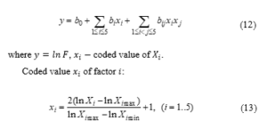
where X_i – natural value of factor i; X_(i_max ), X_(i_min ) – natural values of the upper and lower levels, respectively.

3.3. Design of Multifactor Experiments in the Search for Optimal Technological Conditions and Design Parameters of Equipment.

According to the verified experiment results, it is assumed that on the considered small interval, the response function can be described by a polynomial of the first degree. Due to the linearity of the model, the factors varied at two levels. At the same time, the zero levels were taken on the basis of previous studies [2] (Table 2).
Table 2: Levels of Factors and Variable Intervals

When conducting a full factorial experiment with varying factors at two levels, one replicate of it would involve 25 = 32 experiments. It would make the experiment cumbersome enough if at least three replicates were performed. Therefore, the fractional factorial design of the experiment N= 2^(5-1) was chosen. It reduces the number of experiments of one replicate to 16 due to the system of mixing linear effects of factor x_5 with the least significant interaction effects, but at the same time the number of replicates is increased to three. All experiments, according to the principle of randomization, were carried out in random order. Three replicates for all selected conditions were implemented (Table 3).
Table 3: Experiment Planning Matrix

3.4. Experimental Installation

Experimental Installation has been established (Figure 4). A force-torque sensor 2 (Schunk FT AXIA 80 Ethernet) was installed on the last link of the robot 1. The base bushing 6 is kept in the vibrational device 7, described in [6] and [17].

Figure 4: Experimental installation: 1. Industrial robot ABB IRB 140; 2. The force/torque sensor Schunk FT AXIA 80 Ethernet; 3. Gripper; 4. Triangulation Laser Sensors Riftek RF603.2; 5. The shaft; 6. The bushing; 7. The vibrational device; 8. DC motor; 9. Controlled converter; 10. Electronic frequency meter (Mastech M9803R); 11. The generator of low-frequency oscillations.

The experimental procedure was as follows. The shaft 5 was held by gripper 3 of the robot 1. Vibrations were provided by the original generator of low-frequency oscillations 11. The generator of low-frequency oscillations was controlled by the electronic frequency meter 10, and the actual vibration amplitude of the vibrational device was monitored by contactless laser sensors 4. The first link of the vibrational device performed a rotational motion with a constant angular velocity ω around a vertical fixed axis by a DC motor 8. The DC motor was controlled by a controlled converter 9. All sensor signals were collected and processed by the computer. Thus, during the experiments, continuous monitoring of the current values of technological factors was ensured.
The choice of force/torque sensor Schunk FT AXIA 80 Ethernet was determined by the required process sensitivity. The default value of sensitivity is 0.005 (Where: 0 = no damping – robot maintains speed; 1 = full damping – robot decelerates quickly) and its technical data is presented in Table 4.
Table 4: Technical Data of the Sensor Schunk FT AXIA 80 Ethernet

Storage and Operating Conditions
Storage Temperature [°C]		-20 to +85
Operating Temperature [°C]		0 to +65
Electrical Specifications
Power Source		DC Power
Voltage [V] min. max.		12 30
Maximum Power Consumption [W]		1.5
Measurement Ranges
Parameter	[N]	[N]	[Nm]
Measurement Range 0	500	900	20
Measurement Range 1	200	360	8

 

 

4. Results and Discussion

4.1. Screening of Coarse Observations in Parallel Experiments

For each row of the experiment planning matrix, according to the results of n parallel experiments, y ̅_j – arithmetic mean value of optimization parameter was found:

Where u is the number of parallel experiment; y_ju is the value of the response in the u parallel experiment of the ј row of the experiment planning matrix.
In order to estimate the deviations of the response from its mean value for each row of the experiment planning matrix, the dispersion s_j^2 of the experiment was calculated according to n parallel experiments (Table 5). Statistical dispersion was estimated by an expression of the form:

Table 5: Experimental Results and Dispersion of Forces

 

4.2. Verification of the Uniformity of Dispersions

The dispersion homogeneity was tested by the Fisher F criterion, which is the ratio of the largest to the smallest variance:

where s_1^2 и s_2^2 – respectively, the largest and smallest values of the response variance in different experiments.
If the observed value is F <F_t (F_t is the table value of the criterion F for the corresponding freedom degrees f_1 =n_max-1=2,〖 f〗_2 = n_min -1 = 2 and the accepted significance level of 0.05 [16]) then the variances are uniform (Table 6).
Table 6: Testing the Homogeneity of Dispersion by the Fisher Criterion

With uniform duplication of experiments, the homogeneity of a number of dispersions was checked using the Cochrane G criterion, which is the ratio of the maximum dispersion to the sum of all dispersions:

The dispersions are homogeneous if G< G_t (G_t is the table value of the criterion G for the conditions: N is the number of compared variances N = 16, and n is the number of parallel experiments n = 3 [16]). If G> G_t, then the variances are inhomogeneous, and this indicates that the investigated value y does not obey the normal law (Table 7).
Table 7: Testing the Homogeneity of Dispersion by the Cochrane Criterion

4.3. Determination of Regression Coefficients

According to the results of the experiment, the coefficients of the model were calculated. The regression coefficients are determined by the formulas:

where i,l – numbers of factors; x_ij,x_lj – coded values of factors iand l in the ј-th experiment. These formulas are obtained using the least squares method.
The significance of each coefficient of the regression equation was checked by using Student t-criterion, comparing the obtained values with the table values in the corresponding degrees of freedom and significance level:

If the dispersion s_j^2 of the experiments are homogeneous, the dispersion s_y^2 of the reproducibility of the experiment is calculated by the expression:

Table 8: Significance of each Coefficient of the Regression Equation

	2.975	4.297	1.655	-1.071
	–	0.035	–	0.038
	0.163	0.075	0.101	0.12
	0.053	0.045	0.038	-0.031
	0.396	-0.057	0.265	0.382
	0.045	-0.071	–	–
	0.057	-0.051	–	–
	–	–	–	-0.028
	–	–	–	–
	–	–	–	–
	–	–	–	–
	–	–	-0.044	-0.055
	–	–	–	-0.034
	–	–	–	–
	–	–	–	0.038
	0.04	–	–	–

Student criterion t is calculated for each regression coefficient. Statistically insignificant coefficients can be excluded from (16). The verification results are summarized in the Table 8. The regression equations for the considered response functions y_(F_y ),y_(F_z ),y_(T_x ),y_(T_z ) can be written based on the data given in Table 8.

4.4. Verification of Model Adequacy

After calculating the coefficients of the model and checking their significance, the dispersion of adequacy was determined. The residual dispersion or the adequacy dispersion characterizes the scattering of empirical values of y with respect to the calculated y determined by the found regression equation. The adequacy dispersion was determined by the formula:

where (y_j ) ̅ – arithmetic mean value of the optimization parameter in the ј-th experiment; (y_j ) ̂ – value of the optimization parameter calculated by the model for the conditions of the ј-th experiment; f – the number of freedom degrees; k – the number of factors.
The final step in processing the experimental results was to verify the hypothesis of the adequacy of the found model. Hypothesis verification was carry out according to the Fisher criterion:

If the value F <F_t (F_t – table value of the criterion, F_t = 2.1 for the accepted significance level of 0.05 and the corresponding numbers of freedom degrees f_1 = N- (k + 1)= 16 – (5 + 1)= 10,f_2 = N(n -1)= 32 [16]) then the model is considered adequate. For F> F_t, the adequacy of hypothesis is rejected (Table 9).
Table 9: Result of Model Adequacy Checking

	0.021959	0.003026	0.005974	0.008727
	0.017306	0.003367	0.00647	0.005815
	1.269	0.899	0.923	1.501
	Yes	Yes	Yes	Yes

In this case, we can conclude that the resulting model satisfies the adequacy condition.
For the transition from the coded values to natural values of the factors in the regression equation, values x_i factors on expressions (12) were substituted by (13) and regression coefficients values b_i were referenced in Table 8, obtained:

Potentiating expressions (24 – 27), the dependence of forces and torques on the studied factors of the robotic assembly process was found:

According to (28 – 31), nomograms can be constructed, which allow, for practical purposes, to determine the components of the force and torque acting on the installed part when determining factors for the robotic assembly process.
A suitable response for the above regression model F_z (29) was constructed and nomograms (Figure 5) were constructed with paired combinations of these factors while the other factors were at the zero level.
Figure 5 illustrates the dependence of the force F_z on variable factors in the assembly process. It is clear that the angular velocity and the gap in the joint are inversely proportional to the force F_z, while the vibration frequency, the vibration amplitude and the linear velocity are proportional to the force F_z. Also, there is an interaction effect of two factors of the angular frequency and the vibration amplitude. The maximum value of the force F_z was 87.17 N (Figure 5.f), the minimum value of F_z was 57.86 N (Figure 5. g).
Force F_z decreases significantly with increasing the angular velocity (Figure 5. c, f, h, j). Force F_z decreases rapidly at the initial stage, and then more slowly decreases in the investigated values range of the angular velocity. The maximum value of the force F_z in the absence of the rotational movement was 87.17 N (Figure 5. f), the minimum value of F_z with the rotational movement was 65 N (Figure 5. h). Also, F_z decreases with an increase in the gap in the joint. With the small gap, the maximum value of the force F_z was 84.7 N (Figure 5. j). With the large gap, the minimum value of the force F_z was 57.86 N (Figure 5. g).

Figure 5: Three-dimensional nomograms showing the behavior of force F_z affected by factors of the robotic assembly process.

The force F_z is proportional to the angular frequency and vibration amplitude. The force F_zdecreases with a simultaneous increase or decrease of both these factors (Figure 5. a – Figure 5. g). The angular frequency and vibration amplitude interact with each other, affecting the magnitude of the force F_z. When both factors changed in the investigated values range of them, the change in the value of the force F_z was small (60.8 – 78.3 N) (Figure 5. a). The effect of linear velocity on force F_z is negative (Figure 5.b, e, h, i), however, decreasing the linear velocity the assembly time will increase.

5. Conclusion

The conducted experimental studies revealed the influence of variable factors on the components of the assembly force and torque. Mathematical models that establish the relationship between the components of the friction forces and torques with disturbing factors are formed. The adequacy of the mathematical model of the process is proved. The effects of the interaction of two factors are identified.
The effect of increasing the assembly speed is negative, which correlates with the theory of friction. At the same time, the greatest effect of reducing the assembly force was achieved in the areas corresponding to the lower boundaries of the variation intervals. In various experiments, the decrease in assembly force ranged from 14 to 33%.
The conducted experiments proved the presence of the effect of vibrations and rotation on increasing the technological reliability of the assembly process. Further research will be associated with a change in the zero level of variation of the input factors. It is supposed to check the adequacy of the mathematical model and the results of physical experiments.

Conflict of Interest

The authors declare no conflict of interest.

Acknowledgment

The authors express their gratitude to the Department “Technologies and Equipment of Mechanical Engineering”; Ph.D., Assoc. Prof., Petukhov Sergey Leonidovich, Senior lecturer Mishin Vladimir Nikolaevich and Ph.D., Assoc. Prof., Arkhipov Maksim Viktorovich, Faculty of Mechanical Engineering, Moscow Polytechnic University for the opportunity given to them to work in the laboratory, for significant support and useful suggestions for improving the research.

1. M.V. Vartanov, L.V. Bozhkova, Z.K. Bakena Mbua, “Robot assembly of complex shafts on the basis of passive adaptation and low-frequency vibration”, Russian Engineering Research, 30, 1092–1094, 2010, https://doi.org/10.3103/S1068798X10110055
2. A.L. Simakov, Обоснование методов и средств адаптации соединяемых деталей на базе принципов автоматического управления и выявленных взаимосвязей при автоматизированной сборке, Sc.D Thesis, Kovrov State Technological Academy, 2003.
3. M.G. Kristal, Производительность и надежность сборочных автоматов: монография  – Volgograd: VolSTU, 2011.
4. L.B. Chernyakhovskaya, “Influence of rotational movement of a peg on the automatic peg-in-hole assembly of cylindrical details,” Assembly in mechanical engineering, instrument making, 6, 7-13, 2016 (article in Russian with an abstract in English).
5. L.B. Chernyakhovskaya, Кинематический и динамический анализы автоматической сборки цилиндрических деталей: Монография – Samara: Samara State Technical University, 2011.
6. D.M. Levchuk, Исследование и разработка методов относительного ориентирования сборочных единиц соединения во вращающемся потоке газов при автоматической сборке,, Ph. D Thesis, Moscow Automotive Institute, 1974.
7. Bakšys, J. Bakšys, A. Chadarovičius, “Simulation of vibratory alignment of the parts to be assembled under passive compliance,” Mechanika, 19(1), 33-39, 2013, doi: https://doi.org/10.5755/j01.mech.19.1.3625.
8. Baksys, J. Baskutiene, “The directional motion of the compliant body under vibratory excitation,” International Journal of Non-Linear Mechanics, 47(3), 129–136, 2012, doi: https://doi.org/10.1016/j.ijnonlinmec.2012.01.008.
9. A.A. Ivanov, “Vibration assembly systems,” Assembly in mechanical engineering, instrument making, 5, 7-10, 2013 (article in Russian with an abstract in English).
10. M.G. Kristal, I.A. Chuvilin, “Research of dynamics of internal member lower flank cradle vibrating meshing,” Assembly in mechanical engineering, instrument making, 4, 13-17, 2008 (article in Russian with an abstract in English).
11. V.G. Shuvaev, V.A. Papshev, “Compound oscillatory motion forming device for space orientation of automatically assembling details,” Assembly in mechanical engineering, instrument making, 11, 15-18, 2009 (article in Russian with an abstract in English).
12. A.I. Khuri and S. Mukhopadhyay, “Response surface methodology,” Wiley Interdiscip. Rev. Comput. Stat., 2(2), 128–149, 2010, doi: http://dx.doi.org/10.1002/wics.73
13. A. Bezerra, R. E. Santelli, E. P. Oliveira, L. S. Villar, and L. A. Escaleira, “Response surface methodology (RSM) as a tool for optimization in analytical chemistry,” Talanta, 76(5), 965–977, 2008, doi: 10.1016/j.talanta.2008.05.019.
14. T. Tran, M. V. Vartanov and M. V. Arkhipov, “Application of the Part Rotation Effect for Reliability of the Robotic Assembly Process,” in 2019 International Conference on System Science and Engineering (ICSSE), 25-30, 2019, doi: 10.1109/ICSSE.2019.8823286.
15. Paul, Richard. Modelling, Trajectory Calculation and Servoing of a Computer Controlled Arm [Text] / R. Paul; Translation from English. A. F. Vereshchagin, V. L. Generozov / Ed. E.P. Popova. – Moscow: Nauka, 1976.
16. M.G. Kristal, Обработка результатов планирования экстремального эксперимента, Volgograd, 2019
17. L.V. Bozhkova, M.V. Vartanov, E.I. Kolchugin “Experimental setup for robotic assembly on the basis of passive adaptation and low-frequency oscillations,” Assembly in mechanical engineering, instrument making, 1, 5-7, 2009 (article in Russian with an abstract in English).

(Click Here)

(Click Here)