1. Introduction

It is very important to obtain the forest information timely and correctly for forest management and land cover mapping in forest ecosystems. For example, forest mapping plays an important role in the issues of forest restoration and forest degradation assessment [1]-[4]. Nowadays, it is an effective way to obtain forest structure from satellite image [5], [6]. Hyperspectral image is a typical data of satellite image and widely used in forest mapping because there are lots of spectral bands of this image and beneficial for forest type recognition. What’s more, A series of achievements have been made based on hyperspectral remote sensing technology [7], [8]. However, it leads to the Hughes phenomenon because of redundant spectrum of hyperspectral image [9]. Normally, it needed to be reduced by different methods before image classification [10]. After dimension reduction, traditional classifiers were adopted, such as random forests [6] and support vector machines [7], SVM is the most popular and nonparametric supervised learning method. It is widely used in classifying forest ecosystems [11]. Fortunately, deep learning can extract feature automatically, past studies have showed that deep learning can achieve higher accuracy of image processing of remote sensing avoiding human intervention [12].  Deep belief network is typical model of deep learning.  There is an input layer, one output layer and several restricted in Boltzmann machines [13]. Pre-training and fine-tuning are two important steps in DBN model.  Pre-training is an unsupervised learning from bottom to up and output result with a classifier. Backpropagation was coined by Rumbelhart [14] and used to update the parameter of model for better result.

There are lots of references about image classification using DBN. It seems that DBN was first adopted by Lü et al. in 2014 year [15]. The experiments showed that the optimal network depth was three hidden layers and best nodes of each hidden layer were 64. In year 2015, Chen et al. created DBN model combing with principal component analysis and logistic regression. They confirmed better effect of DBN than that of SVM [12] adopting two Hypersperctral datasets, such as Indian Pines and University of Pavia. On the whole, there are a lot of application situation of deep learning [16], but few literatures is reported about forest mapping using deep learning from Hyperspectral image.

Therefore, one of our research objectives is to confirm the performance of forest mapping by DBN using hyperspectral data. Another objective of this study is to compare the classification performance of DBN model and SVM algorithm. Third objective is to investigate how optimal parameters of DBN affect overall accuracy and Kappa coefficient of forest type identification. The major contribution is to determine the optimal parameters of DBN for forest mapping from Hyperspectral data.

2. Methods

2.1. Restricted Boltzmann Machines (RBM)

RBM is a directionless, full connective model [17]. A RBM consists of two layers. One of them is an input layer, or visible units v. Output layer, or hidden units h  is another layer of RBM. There are no connections within each layer. From Figure 1, we know that the units between visible and hidden are full connected by weight W. The energy of a joint configuration with v visible units and h hidden units is

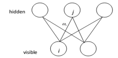
Figure 1: The model of an RBM

Where  represents parameters of RBM. is the weight between input layers i and hidden layers j.  is the bias of ,  is the bias of . I and J are total numbers of input and output layers respectively. The probability of the joint configuration over both layers is

where  is the normalized factor, equals to .

    In the binary case where , given input layer, a conditional probability of an output layer being 1 is given as:

    In the same way, the conditional probability of input layer given the output layer:

where the  stands for the true outputs,  corresponds real outputs. In general, there are K outputs. Gradient descent is a good method to minimize total error, it is ecessary to compute the partial derivative of E with respect to each weight in the network. The parameters, such as weights and biases will be iterated by stochastic gradient ascent which can be formulated as [18]:

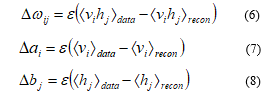
where  is a key parameter, that is learning rate.  is expectation for data distribution and  is the expected value of the model distribution.

2.2. Deep Belief Network

Several RBMs stacked into a classical model of deep belief network. There are two important steps in the DBN [19]. One is pre-training and the other is fine-tuning, shown in the Figure 2. Initial parameters are produced in the pre-treatment by an unsupervised method, such as gradient descent method to avoid local optimum. Back-propagation is normally used to update model parameters according to error, such as squared error or cross entropy error.

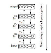
Figure 2: A generative model of deep belief network

2.2.1. Pre-training

Pre-training of DBN model is an unsupervised procedure. At the beginning, the input layer is initialized to a training vector. Then the subsequent hidden layer of RBM is trained through the output of the previous layer. Moreover, this whole process can be repeated until the final hidden layer. By doing so can the DBN extract more and deep feature from the original input data.

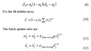
2.2.2. Fine-Tuning using Backpropagation algorithm

Backpropagation was coined by Rumbelhart [20]. Backpropagation update model parameters using cross entropy error because there is four kinds of outputs in this paper.

2.3. Indicators of Evaluation of Classification

·         Overall accuracy

The overall accuracy is total assessment of classified quality, which equals the total pixels sum divided by correctly classified pixels by total pixels. The formula for calculating the overall accuracy based on the confusion matrix can be listed as following:

here, C represents the number of categories, and represents the elements on the diagonal of the confusion matrix, and N represents the total number of test samples.

• Kappa coefficient

Kappa coefficient adopts a multivariate discrete analysis technique to reflect the consistency between classification results and reference data. It considers all factors of the confusion matrix, and it is a more objective evaluation index, which is defined as:

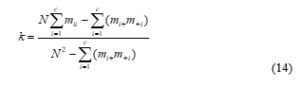
Among them, and represent the sum of the line i of the confusion matrix and the sum of the column i respectively. The higher the Kappa coefficient, the higher the classification precision.

3. Data and Process

3.1. Study site and hyperspectral data

Hyper Spectral Imager (HSI) is the first Chinese space-borne hyperspectral sensor aboard the HJ-1A satellite. In September 6, 2008, China launched the environmental and disaster monitoring and forecasting small satellite constellation A (HJ-1A), and the HJ-1A satellite was equipped with CCD camera and hyperspectral imager (HSI). With HSI interference imaging spectroscopy, the cutting width is 50km, the ground pixel resolution is 100 meters, 110-128 spectral bands, the spectral resolution of up to 2.08 nm, in the continuous spectral image of earth observation and available features to achieve the direct identification from the space object surface. HSI often produces certain stripe noise on the image. Satellite data was HJ-1A star HSI data 2 level products, imaging time is August 24, 2011, a total of 115 bands with working spectrum range 459 ~ 956 nm.

The research area has 8 downtowns in the west of Dehua county, Quanzhou City, Fujian Province. The administrative area of study site and its pseudo color synthetic imaging (105th, 7th, 40th band for pseudo colour synthesis) are shown in Figure 3. The image data of the product is geometrically corrected by previously corrected image with polynomial transform, and then orthorectified and outputted onto a fixed uniform spatial grid using nearest neighbour resampling. The correction error is not less than one pixel. The corrected image is unified into the specified map projection coordinate system (Xi’an 1980 coordinate system). There is obvious stripe noise in the part of the HSI image data, mainly in bands 1-29. Therefore, these 29 bands are eliminated from the HSI image. The remaining 86 bands are used for research within the wavelength range (529.6350-951.54 nm).

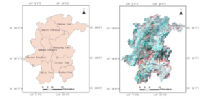
Figure 3: Study area and pseudo colour synthetic image

3.2. Experimental processing flow

According to the field data, the labelled samples were selected in the experiment. Then 86 bands of data were used as input of DBN. Before the training, these data were normalized by min-max normalization, which was mapped into the value between 0 and 1. Then, these data were shuffled and split into training and testing data randomly. After pre-training and fine tuning, categorical data was represented by one-hot coding, as shown in Table 1, 1 was Coniferous forest, 2 was Broad-leaved forest, 3 was Mixed forest, 4 was Non-forest.

The experiment is based on Windows 10 with 64-bit operating system. The processor is Intel (R) Core (TM) i5-8250U CPU @1.60GHz. The experiment is carried out in PyCharm 2018.3×64 editor to code and tune parameters. TensorFlow 1.11.0 framework was first set up as development environment. Also, The Python Extension Library is loaded, including Numpy, Pandas, Matplotlib, etc.

Then the selected samples were converted into a CSV file that is easy to be processed by Python program. All these samples were shuffled into training and testing data. Moreover, training samples were thrown into the DBN model. The trained parameters of model were stored into Tensorboar. Finally, the classified map of was outputted.

3.3. Distribution of samples

There are total 97258 pixels in the pseudo color synthetic image, shown in Table 1. The samples of four types in study site are selected manually. Different allocation of training samples and test samples are selected by experiments again and again. At last, 28000 pixels of known categories were selected as total samples. Among them, 51989 pixels pertain to the coniferous forest, 6142 pixels are broad-leaved forest, 16283 pixels are mixed forest, and the remaining 28986 pixels are non-forest. In the training process, there are 10,000 training samples for coniferous forest and 6,000 training samples for other forest type.

Table 1: Class code of dataset

Code of label	Forest type	Number of training samples	Number of testing samples	Number of all samples
1	Coniferous forest	10000	4000	45848
2	Broad-leaved forest	6000	4000	6142
3	Mixed forest	6000	4000	16283
4	Non-forest	6000	4000	28985
	total	28000	16000	97258

4. Experimental Results

4.1.  Selection of super parameters

In the experiment, the dimension of the input data is 86. At the moment, network structure of DBN model is only designed by experience without theoretical basis. For simplicity, we assume that each hidden layer has the same number of nodes. The number of layers of the DBN is selected from {2, 3, 4, 5, 6, 7}, and the number of hidden layer nodes is selected from {16, 32, 64, 128, 256, 512}. According to the pre-experiments and references, several parameters are set as following: pre-training and fine-tuning of the learning rate is 0.001, the size of mini-batch is 100. Note that 10000 iteration times are run due to stability. Next, we discuss the influence of different network depth and the number of hidden layer nodes on the classification effect by fixing all these super parameters.

4.2. Network depth

Overall accuracy (OA) and Kappa coefficient were normally selected as the evaluation of image classification of remote sensing.  The higher OA and Kappa coefficient, the better effect of classification precision. As we all know, network depth is key parameter of DBN. It is the number of hidden layers. Reference 21 summarized the range of optimal network depth is from 2 to 3 based on previous researches.

In experiment, we keep super parameters fixed and set the number of nodes in each hidden layer 256.  Six different numbers (2, 3, 4, 5, 6, 7) of network depth were tested. Figure 4 shows that DBN with 3 hidden layers performs best, which both overall accuracy and Kappa coefficient are the largest. There is no obvious feature that how network depth affects the OA and Kappa coefficient. Reference [21] pointed out that there is no perfect theoretical basis for network structure selection. The optimal parameters should be given by experiments in different applications.

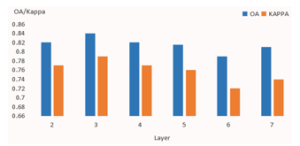
Figure 4: Effect of network depth on OA and Kappa coefficient

4.3. Number of nodes in each hidden layer

Number of nodes in the hidden layer is also import parameter in DBN model. When nodes are too large, it may cause the over-fitting problem. Oppositely, when nodes are too small, perhaps it will fail to extract deep information and gain high classification accuracy. Summarized by reference 21, the range of number of nodes in the hidden layer is from 50 to 500 according to previous research.

In experiment, we set super parameters unchanged and keep the network depth 3.  Six various nodes (16, 32, 64, 128, 256, 512) were selected one by one and tested. Effect of number of nodes in each hidden layer on OA and Kappa coefficient is showed in Figure 5. It demonstrates that DBN with 256 nodes performs best, because it got the biggest overall accuracy and Kappa coefficient.

There is no obvious feature that how network depth affects the OA and Kappa coefficient. Reference [21-24] pointed out that there is no perfect theoretical basis for network structure selection. The optimal parameters should be given by experiments in different applications. Meanwhile, OA and Kappa coefficient keep relatively stable with changing nodes.

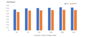
Figure 5: Effect of number of nodes in each hidden layer on OA and Kappa coefficient

4.4. Comparative analysis

SVM is a supervised and non-parametric machine learning algorithm. There is different type of kernels. A radial basis function (RBF) was adopted and has been used in some former works concerning forest type classification. The penalty factor C is selected from [1, 0.1, 0.001]. In order to keep the equit, the same samples are adopted between SVM and DBN method. Furthermore, to optimize of SVM method, five-fold cross validation and network search are adopted. When the C value is 1, the maximum overall accuracy is 73%, and the Kappa coefficient is 0.6447. For deep belief network, the optimal number of network depth is 3 and number of each node is 256.The classification process resulted in a thematic map of four kinds of forest types in Dehua county, as shown in Figure 6. As can be shown, the coniferous forest is green, broad-leaved forest is yellow, mixed forest is pink, and non-forest is blue.

Table 2 reports the kappa values and the accuracy of forest types for both DBN and SVM classification algorithms. The accuracies of four kinds of forest types for SVM oscillated between 0.64 and 0.74 while DBN method varied from 0.82 to 0.89. Hyperspectral image classification using DBN algorithm yields the higher accuracy than that of SVM classifier for each forest type. Broad-leaved forest was generally better recognized than coniferous forest. Broad-leaved forest is classified with highest accuracy for both methods, 0.92 for DBN, while for SVM it is 0.84. The second top-classified forest type tends to be non-forest for DBN, while for SVM it is coniferous forest. Slightly lower result is obtained for mixed forest by DBN, while for non-forest by SVM. Furthermore, the worst effect performed by DBN algorithm is coniferous forest, compared to mixed forest for SVM. As the result, DBN model tends to attain better capability than SVM method from accuracy. There are two reasons due to it. One is that all feasible spectral features are thrown into input of DBN model, yet three bands or several components are selected as input for SVM method. The other is that there is large amount of data when all hyperspectal bands are considered. This is good for training of DBN model.

5. Conclusion and Discussion

This paper examined the capability DBN model in forest type classification with HJ/1A hyperspectral image. Many experiments are tested to obtain optimal parameter in DBN model. Conclusions can be drawing out as followed. At the beginning, the results showed that DBN model outperform SVM algorithm. Then, optimal network depth is 3 and best node in each layer is 256 in our experiment. Overall accuracy is 85.8% and kappa coefficient is 0.785 with best-fit parameters in DBN model.

Table 2: Comparison with SVM

Forest type	SVM	DBN
coniferous forest	0.74	0.82
broad-leaved forest	0.84	0.92
mixed forest	0.64	0.87
non-forest	0.70	0.89
OA	0.73	0.875
Kappa	0.6447	0.835

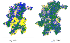
Figure 6: Comparison of classification results based on different machine learning techniques

What makes our study unique is to make use of deep belief network to classify the forest type. Regardless of the spatial resolution of 100 m of HJ/1A hyperspectral image, our results provide satisfied recognition of four kinds of forest types. There are several open questions and future research directions remain worthy of investigation in the future. Firstly, in this paper, it is novative to adopt deep belief network to identify forest types. The classification accuracy of this method are better than that of support vector machine. However, it is still unclear that the mechanism of how this method can solve the traditional problem of “same object with different spectra” and “same spectra with different object “. Secondly, our results confirm the capability to map forest by deep belief network. Our experience in the study reveals that network depth and width affect accuracy of classification. The optimal structure needed to be adjusted according to different remote sensing data and further identification, such as tree species mapping. Finally, combining with field survey data, nearly one third of the samples are selected as training and testing samples to improve the classification effect. It is uncertain that how can we obtain the best result with so high number of total samples. It is a good idea to expand the sample by Generative Adversarial Network. Last but not least, optimal network structure is only for forest type recognition. The optimal network structure of specific forest type recognition needs further study. At the same time, it is urgent to establish the criteria and norms of forest classification using deep learning and remote sensing image.

Conflict of Interest

The authors declare no conflict of interest.

Acknowledgment

The work was supported by the Project of Natural Science Foundation of Fujian Province under Grant No. 2020J01785, the project from the department of Quanzhou Science and Technology under Grant No. 2016N057 and the project from the department of education under Grant No. JAT170475. The author gratefully acknowledges the support of K.C. Wong Education and DAAD (No. 91551268). The authors also acknowledge the support by Fujian Provincial Key Laboratory of Data-Intensive Computing, Fujian University Laboratory of Intelligent Computing and Information Processing, and Fujian Provincial Big Data Research Institute of Intelligent Manufacturing.

1. G. Modica, A. Merlino, F. Solano, R. Mercurio, “An index for the assessment of degraded Mediterranean forest ecosystems”, Forest Systems, 24, 1-3, 2015, doi:10.5424/fs/2015243-07855.
2. X.G. Kang, “Forest Management”. Beijing: China Forestry Publishing House, 10-28, 2011.
3. I.D. Thompson, M.R. Guariguata, K. Okabe, et al, “An operational framework for defining and monitoring forest degradation”, Ecology and Society, 18(20), 2013, doi: 10.5751/ES-05443-180220.
4. L. Kurvonen, M.T. Hallikainen, “Textural information of multi-temporal ERS-1 and JERS-1 SAR images with applications to land and forest type classification in boreal zone”, IEEE Transactions on Geoscience and Remote Sensing, 37, 680-689, 1999, doi:10.1109/36.752185.
5. Mei, A. X., Peng, W. L., Qin, Q.M. et al. “Introduction to remote sensing”. Beijing: Higher education press, 225-286, 2006.
6. A. Ghosh, F.E. Fassnacht, P.K. Joshi, B. Koch, “A framework for mapping tree species combining hyperspectral and LiDAR data: Role of selected classifiers and sensor across three spatial scales”. International Journal of Applied Earth Observation and Geoinformation, 26, 49-63, 2014, doi:10.1016/j.jag.2013.05.017.
7. Y.Y. Dian, Z.Y. Li, Y. Pang, “Spectral and Texture Features Combined for Forest Tree species Classification with Airborne Hyperspectral Imagery”. J Indian Soc Remote Sens, 43(1), 101-107, 2015, doi:10.1007/s12524-014-0392-6..
8. N. Puletti, N. Camarretta, P. Corona, “Evaluating EO1-Hyperion capability for mapping conifer and broadleaved forests”. European journal of remote sensing, 157-169, 2016doi:10.5721/eujrs20164909.
9. G. Hughes, “On the mean accuracy of statistical pattern recognizers” IEEE transactions on information theory, 14(1), 55-63, 1968, doi:10.1109/TIT.1968.1054102.
10. R.E. Faßnacht, “Assessing the potential of imaging spectroscopy data to map tree species composition and bark beetle-related tree mortality”. Freiburg: Freiburg university, 1-20, 2013, doi: 10.1016/j.rse.2013.09.014.
11. M. Mustafa, A.R. James, S.J. Karl, R. David, M. Charles, “Remote Distinction of A Noxious Weed (Musk Thistle: CarduusNutans) Using Airborne Hyperspectral Imagery and the Support Vector Machine Classifier”. Remote Sensing, 5(2), 612-630, 2013, doi: 10.3390/rs5020612.
12. Y.S. Chen, X. Zhao, X.P. Jia, “Spectral-spatial classification of hyperspectral data based on deep belief network”. IEEE Journal of selected topics in applied earth observations and remote sensing. 1-12, 2015, doi:10.1109/JSTARS.2015.2388577.
13. E. Alpaydin, Introduction to machine learning(third edition), The MIT press, 267-311, 2014.
14. L. Deng, S.S. Fu, R.X. Zhang, “Application of deep belief network in polarimetric SAR image classification”. Journal of image and graphics, 21, 933-941, 2016, doi: 10.1109/IGARSS.2015.7326284.
15. Q. Lü, Y. Dou, X. Niu, J.Q. Xu, F. Xia, “Remote sensing image classification based on DBN model”. Journal of computer research and development. 51, 1911-1918, 2014, doi:10.7544/issn1000-1239.2014.20140199.
16. P. Zhong, Z.Q. Gong, S.T. Li, et al., “Learning to Diversify Deep Belief Networks for Hyperspectral Image Classification”. IEEE Transactions on Geoscience and Remote Sensing, 1-15, 2017, doi:10.1109/TGRS.2017.2675902.
17. G.E. Hinton, J.S. Terrance, Learning and relearning in Boltzmann machines. MIT Press, Cambridge, 282-317, 1986.
18. H.M. Xie, S. Wang, K. Liu, S.P. Lin, B. Hou. “Multilayer feature learning for polarimetric synthetic radar data classification”. in IEEE International Geosicence and Remote Sensing Symposium. 2818-2821, 2014, doi: 10.1109/IGARSS.2014.6947062.
19. G.E. Hinton, R.R. Salakhutdinov. “Reducing the dimensionality data with neural networks”, Science, 313, 504-507, 2006, doi: 10.1126/science.1127647.
20. L. Deng, S.S. Fu, R.X. Zhang. “Application of deep belief network in polarimetric SAR image classification”. Journal of image and graphics, 21, 933-941, 2016, doi:10.11834/jig.20160711.
21. C.C. Yao, X.X. Luo, Y.D. Zhao, et al, “A review on image classification of remote sensing using deep learning” in Proceedings of 2017 3rd IEEE Internaitonal Conference on Computer and Commmocaotpms, 1947-1955, 2017, doi: 10.1109/CompComm.2017.8322878.
22. S.J. Ge, J. Lu, H. Gu, et al., “Polarimetrie SAR image classification based on deep belief network and superpixel segmentation.” in 2017 3rd International Conference on Frontiers of Signal Processing, 115-119, 2017, doi: 10.1109/ICFSP.2017.8097153.
23. M.M. Lau, J.T.S. Phang, K.H. Lim, “Convolutional Deep Feedforward Network for Image Classification.” in 2019 7th International Conference on Smart Computing & Communications, 2019, doi:
24. A. Mughees, L.Tao, “Multiple Deep-Belief-Network-Based Spectral-Spatial Classification of Hyperspectral Images.” Tsinghua Science and Technology 24(2), 183-194, 2019, doi: 10.26599/TST.2018.9010043.

(Click Here)

(Click Here)