1. Introduction

Energy wastage is still an enormous problem around the world, even about 40% due to inefficient city building energy management systems [1,2]. Challenges in the recent energy industry are cost-effective deficiencies, model inaccuracy, and lack of prediction procedures determining the use of energy that can be measured periodically to make significant decisions [3]. Investors have invested a lot of money to improve sustainable building’s energy efficiency to reduce costs and emissions. The question is whether energy efficiency has worked success  effectively reducing energy consumption to the maximum? Then the next question is how effectively the method works in the influence of various external factors? In previous research on energy efficiency, it concluded that the best strategy is not only to apply energy-saving technology. But energy management strategies can also be an effective solution in minimizing energy disposal [4].

Energy benchmarks are still a consideration for building owners to be able to measure the energy consumption performance of building with similar structures to different geographical or weather conditions. Based on the results of energy benchmark analysis, building developers can implement appropriate and proven energy-saving methods by the best practice of other buildings. The core keys to knowing the maximum energy savings are by determining the energy demand model before the development action (baseline model) and determining the energy demand prediction model after the implementation of the energy-saving method (report model) [5]. Meanwhile, the new energy benchmark introduced in California Energy Policy for verifying the success of energy-saving in 2017, namely NMEC.  The NMEC considers the weather and building characteristics to normalize energy consumption data. Normalization indicates a statistical process for adjusting energy use before and after energy management improvements in a wide range of conditions related to independent variables for more sensible results that can describe actual energy consumption patterns [6].

Previously researchers successfully used the Hybrid model Artificial Neural Network (ANN) with an average Mean Absolute Percent Error (MAPE) value of 4.2% [7]. On the other hand, the model still has limitations where it can give a decent prediction for only the next 72 hours. Another research uses LSTM performs well in terms of accuracy, but it requires more data compared to other methods [8]. Until now, various algorithms have been explored widely for predicting building energy consumption. However, many external factors such as holidays or high season trends that change occasionally in many cases, which cannot capture by models. And it’s hard practically to produce feasible analysis results for many business users.

In this research, the authors had the idea to implement the Prophet method to predict building energy use based on historical trends that address dynamic business needs and require time efficiency. Prophet demonstrates higher accuracy and ease of implementation to see movement trends periodically for business purposes with flexible requirements after studying the evaluation results in several previous studies such as Autoregressive Integrated Moving Average (ARIMA) [9], and Seasonal Trend Decomposition using LOESS (STL), ARIMA, Neural Network Autoregressive (NNAR), Trigonometric Exponential Smoothing State-Space model with Box-Cox transformation (TBATS), Linear, S. Naïve in [10]. Prophet can also effectively solve the problem of easy forgery using real-time prediction of the user behavior to determine the right time to switch on the security sensor on the smartphone [11].

We believe that there are still fewer applications for prophet methods, especially in predicting energy consumption in buildings. Although it is still new development methods, the prophet method can surpass various other approaches with the concept of an additive model to estimate predictions based on historical trend patterns. For further development, the authors combine affecting normalization techniques to improve the quality of the model. The purpose of the research will later contribute to producing baseline models that can minimize external effects (e.g., weather, building characteristics, etc.) as an accurate evaluation model of building energy savings in the future. And it could be a consideration for investors to prepare a strategy for the implementation of high-value prolonged energy savings.

2. Literature Review

2.1. Energy Consumption Performance Indicators

Factors that affect energy consumption in buildings generalized into 7 categories [12]:

• Weather (g., air temperature, wind speed, solar radiation, humidity),
• Building characteristics (g., building functionality, square area, number of floor levels),
• Characteristics of occupants (g., presence of residents on weekdays and holidays),
• Building service system (g., cooling/heating conditions, availability of water heaters),
• Activities and habits of residents (g., turning off lights during the day),
• Social and economic factors (g., education level, energy cost), and
• Needs for indoor air temperature.

The behavior and habits of the occupants are quite difficult parameters to identify regarding the complexity and differences of each occupant observed [12]. One of the most possibles solutions is to use real measurement data such as historical data on KWH electricity usage of the previous period. Based on four energy consumption performance methodologies on buildings explained in [13], we chose to use statistical analysis (regression model-based) as the best option to overwhelm the time limitation problem. Statistical analysis methodology refers to the measurement of Energy Performance Intensity (EPIs) in buildings derived from a combination of supportive variables with robust relationships to energy usage.

2.2. Structure Dependent Energy Usage /Loss (SDE U/L) Overview

Energy consumption estimates in buildings usually consider dry-bulb temperature, known as normalization of weather Heating and Cooling Degree Days (HDD/CDD) [14]. HDD/CDD is the standard term of measurement units for conducting weather modeling. However, this method can provide misleading solutions because unable to keep up with the dynamics of extreme weather changes by limited inputs and ratio concept. The development of this method continued to be carried out throughout until recently the SDE U/L method introduced to the public. The SDE U/L method uses the concept of linear or nonlinear models considering the coefficients of wind speed, humidity, radiation, and outdoor temperature. Moreover, several important building factors such as building size, window size, construction connection that ignored in the application of various previously normalization methods [15]. SDE U/L consists of 3 main factors, namely weather, characteristics of buildings, and behavior or habits of building occupants.

In steady-state, (1) represent linear models to calculate the heat balance of the building denoted by g_bl(·) function. The equation made base on heat/cool generated by building appliances that improve overall electricity use. Coefficients a, b, c, and d are parameters that depend on the building’s characteristics. Parameter a relates to insulation, building size, etc. that affect air temperature. Parameter b associates to the direction of entry of sunlight, the size of the window, the material of the window that affects the intensity of radiation. While parameter c is related to air ventilation, the height of the building, the open space that affects wind speed. And parameter d relates to the infrastructure that affects the humidity of the room. Parameter e could consider as the number of residents of the building. While non-linear models have the same concept as linear models, but the application of methods developed with Multi-Layer Perceptron. Where each input node consists of T, R, W, H, P, and when the data do not exist, then the node input will be omitted. The model is optimally attached when the RMSE result is smaller than 10^-10.

2.3. Prophet Overview

The prophet method concept is adapting the Generative Additive Model (GAM) method that emphasizes regression models with non-linear smoothers on the regressor [16]. As a difference, Prophet only uses time as a regressor when there is the possibility of some linear and non-linear functions of time as essential components. Prophet can generally meet the main criteria of good time series models described further in [17] such as forecasting, modeling, and characterization. One of the advantages adapted from the GAM model is the flexibility in accepting trend changes in the data source and quickly in the process of model fittings so that users can change the parameter model interactively to improve accuracy results [18]. Prophet’s model base on the concept of a decomposable time series with three main components: trend, seasonality, and holidays that represent in (2) [19]. The additive regressive model result of combination decomposable time series denotes as y(t), which will describe per movement how the Prophet model fits data distribution.

In (2), g(t) describes the trend of non-periodic changes in the time series model. s(t) describes periodic changes such as weekly, yearly. And h(t) depicts the continued effect of holidays on a nation that has the potential to cause unusual trends and sometimes effects occurring over one day. Notation errors are distinct changes that the model cannot predict. The fundamental in a decent non-linear model is to make sure the model can describe the growth trend and how the continuation corresponds to the addition of data. With dynamic trend movements, the basic approach used is the logistic growth model follows in (3).

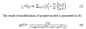
C represents carrying capacity, k is the growth rate, and m is the offset parameter. Carrying capacity is the maximum number of individuals that can be supported resources in an ecosystem. One of the modifications implemented in the Prophet method is to define changepoints, which variable C changes to C(t) defines carrying capacity expected at any given time. Then Prophet defines a vector containing a rate adjustment of δ ∈ R^S, where δ_j is the change in the rate at the time of s_j. Then base k will be couple with adjustment at that point:  k + a(t)^Tδ. Where vector a(t) – {0, 1^S is defined in (4) to limiting that the k rate increase will only occur when the t measurement time exceeds the changepoint time occurred.

The k rate variation is also followed by an offset parameter change to connect the endpoints of the segments. The correct adjustment at changepoint j is easily computed as and presented as follows in (5):

In determining the changepoint on the model, the analyst can perform manually by defining a specific potential signifiant date as an example of a national holiday. Or automatic by applying the principle of historical trends to variable δ and sets the flexibility rate in the model by parameter _T. For the record, the application of historical trends in δ will not influence the central point growth rate of k. Thus, when the parameter _T value is 0, the curve of the fitting model will be linear or basic logistics. Accuracy in the prediction model becomes the final parameter as the evaluation material, but the error value of uncertainty would still occur due to the unconstant growth rate. Uncertainty calculates assuming that future predictions will have an average pattern of frequency and enormous changes in growth rates in history. To increase accuracy, we can configure the _T parameter based on the variant result of the data. The increasing value of the _T parameter will also increase the flexibility of the model fitting to historical patterns and reduce the error loss value. However, high flexibility is directly proportional to the increased interval of uncertainty.

In the Prophet model, the seasonal component s(t) provides adaptability by permitting periodic changes in a different kind of seasonality. There are many cases of multi-period seasonality as a capture result of human behaviors. For instance, a 5-days workweek implies effects on a time series that repeat each week for over a month, while vacation schedules at the weekend and school breaks can generate a trend that repeats each year. To fit and forecast these effects we must specify seasonality models that are periodic functions of [time] t. Prophet relies on the Fourier series to provide a lenient model of periodic effect. P is the regular period the time series will have (e.g., P = 365.25 for yearly data or P = 7 for weekly data when time scale in days).

The impact of a particular holiday on the time series is often similar year after year, making it important incorporation into the forecast. The component h(t) indicates predictable events of the year including those on irregular schedules (e.g., Halloween or Labor day). To utilize this feature, the user needs to provide a custom list of events. Fusing this list of holidays into the model is made straightforward by assuming that the effects of holidays are independent. After the model fitting process, the model will make predictions based on trends and seasonality that successfully captured previously in (1). Trend assumptions are based on the same date in the previous period. The output of the model will be yhat variables that indicate the predicted results. And another component yhat_lower and yhat_upper, which describes uncertainty intervals of prediction.

2.4. Related Works

In this section, it will explain in more detail about the methods used along with the evaluation results obtained by the previous research. Previously researchers used four approaches as a comparison to create baseline models of energy prediction such as Support Vector Machine (SVM), Long Short-Term Memory (LSTM), Nonlinear Auto-Regressive (NAR), Autoregressive Moving Average (ARMA) [8].  It could conclude that each method tested can exceed ARMA performance. While LSTM performs well in terms of accuracy, it requires more data compared to other methods. Hybrid model Artificial Neural Network (ANN)-based Short Term Load Forecasting (STLF) models with a combination of boolean metering systems to convert input values into vector bit shapes carried out in [7]. The experiment conducted using energy consumption data on 93 homes in Portugal from 2000 to 2001. The experiment proved a pretty good result with an average Mean Absolute Percent Error (MAPE) value of 4.2% as well as a maximum MAPE of 18.1%. In the evaluation results, there are limitations where the model can give a decent prediction for only the next 72 hours. They suggest further development with variable use of air temperature and weather and consider the presence of residents by distinguishing routines on weekdays and weekends to improve the accuracy of prediction models. Other research with the concept of short-term load forecasting for the next 24 hours had a comparison between ANN and SVM methods, with an accuracy rate of 62% for ANN and 60% for SVM [20].

Another comparison method based on a data-driven approach on two buildings to get predicted results of energy consumption per hour meet the model calibration criteria defined by the American Society of Heating, Refrigerating, and Air-Conditioning Engineers (ASHRAE). Various methods such as multiple linear regression, adaptive linear filter algorithms (least mean square (LMS), normalized least mean square (nLMS), and recursive least square (RLS)), and Gaussian mixture model regression (GMMR) used in this experiment [21]. Once evaluated, the GMMR method can go beyond a variety of other adaptive approaches. Cause GMMR is a non-linear method so it can better show the performance of building energy consumption. For an additional record, the data-driven method’s large number of parameter inputs does not ensure better accuracy. It is due to the model’s difficulty in achieving a convergence state in finding the best solution due to the combinatorial explosion problem. Table 1 shows the summary of related works, together with the dataset, method, and achieved experiment results.

Table 1: Summary of Related Works

Ref	Dataset	Method	Result
[7]	Energy Consumption  on 93 Homes in Portugal	Hybrid ANN	Gives an average MAPE around 4.2 %.
[8]	Power Consumption for a Single Household.	SVM	NAR worked best for short time error variance progress while SVM best for long prediction intervals.
		LSTM
		NAR
		ARMA
[20]	Power Consumption for a Single Household in Poland.	ANN	ANN worked best with an accuracy around 62 % for short-term load forecasting.
		SVM
[21]	Buildings Energy Consumption.	MLR	GMMR give best result on fitting building energy consumption model
		LMS
		nLMS
		RLS
		GMMR

3. Experimental Design

In this section, we describe the framework that we used to perform data normalization until the implementation of prediction methods for a group of buildings with the same characteristics as the comparison with other groups. Moreover, we explain the steps and configuration parameters for the numerical assessments of Section 4.

3.1. Dataset

The data in this experiment consists of 3 datasets: weather, electrical consumption of buildings, and building characteristics.

Dataset acquires from meter measurements of more than a thousand structures across the United States [22]. The data consist of measuring water, electricity, gas, hot water, and steam meters. ASHRAE’s 1000-building electrical energy consumption data has an hourly interval with a measurement period from 2016 to 2017, thus meeting the regularly spaced criteria in the time series. Once the data are collected, the data going through the selection phase since some buildings do not have full sensors or there might construction conditions in certain areas, possibly making the sensor measurement value 0.

In ensuring a valid measurement where the building is inhabited, then the maximum missing data is set at 15%. Besides, missing values are replaced with a value of -999 or with interpolation automation techniques based on data of the previous and next day. To eliminate outliers on data, the plot analysis method used in looking at the trends of each district’s building sensors. In this simulation, one building was randomly selected with an N/A value of less than 10 percent to provide the best results. The historical movement of energy consumption over a year with hour intervals could be seen in Figure 1.

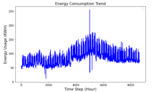
Figure 1: Electrical Energy Consumption Trend on Building with Id 1082.

3.2. Weather Normalization

Then in the stage of weather normalization, implementation is carried out by SDE U/L method to consider meter measurement with weather conditions as well as building characteristics as inputs. Normalization has done using a multi-layer perceptron with configuration four input nodes, two hidden layers, and one output node. For the normalization process, the base temperature sets to 9.6°C, which refers to the average temperature of the building area on measured year. The configuration of base variables used in normalization could be different depends on the needs of research in analyzing the most influential weather factors for the development of energy-saving methods in the future. The trend of electricity consumption after normalization could be seen in Figure 2. Differences in radiation normalization results through the same data could be seen in Figure 3. Because there is no additional information about the behavior of the occupant, thus the input node in parameter P be ignored on the model. For the final training model configuration, we use two hidden layers with each consisting of seven nodes and a learning rate of 0.04.

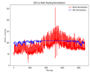
Figure 2: Temperature Base Normalization Implementation.

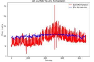
Figure 3: Radiation Base Normalization Implementation.

3.3. Prophet Framework

Preparation of the prophet prediction model carried out in the following stages:

• Split data into three sets, training set, validation set, and test set. The proportion we used in splitting the dataset into training, validation, and test sets is 80%, 10%, and 10%, respectively as a reasonable option given the sufficient amount of data [23]. Training sets were used to train models, while validation sets were used for tuning hyperparameters, and test sets were used for evaluation of models.
• Initialize the carrying capacity value for each row of data presented in the stamp column. The stamp value is not continuously adjusting to the market size at the time of measurement. The market size here refers to the maximum amount of energy consumption per hour. Therefore, carrying capacity plays a role to keep the curve of the model does not exceed the market size value specified before. For example, in the winter season (December – February), the carrying capacity value is determined based on the maximum value of energy consumption between those three months. For the implementation of carrying capacity, minimum value can be used floor variable.
• Defines specific dates such as national holidays that repeat periodically for each year in the form of data frames like Christmas, labor-day, etc.
• Add custom seasonalities such as school holidays in the long-term summer holidays for up to 3 months.
• Change the changepoint ratio on the model to set the flexibility of the model. By default, change points have automatically added to 80% of trends with the reason for creating more projection lines so that there is no overfitting at the end of the prediction. But to be aware, adding a changepoint ratio will make the model have too much flexibility and have overfitting side effects. The default changepoint ratio value in the Prophet method is 05.
• Apply fouries series yearly seasonality tuning as a smoothing method when trend patterns have high fickle frequencies. For example in tropical conditions, the weather changes rapidly.
• Divide the data into 2 columns, ds for the date (timestamp) and y for the feature column which is the result of normalization of building energy consumption as input in the model.
• Repeat steps e through f to find the best model through a final evaluation using RMSE.

3.4. Evaluation Metrics

For the final evaluation, we used simulated historical forecasts (SHF) that relate the concept of the cross-validation method by calculating the average RMSE predicted results made periodically over the specified time frame. In this simulation, the model will be fitted with the initial data of 10 months and make predictions for each week within the next two months. An overview of the cross-validation periods section could be seen in Figure 4.

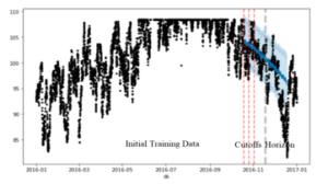
Figure 4: Cross Validation Periods.

3.5. Environment and Parameter Setting

These experiments were conducted on Google Colab using GPU accelerator with Python programming language. The models created using the Prophet forecasting model through the logistic growth model as a trend factor base. The final configuration of the Prophet model in this experiment could be seen in table 2.

Table 2: Prophet Parameter Setting

Parameter	Setting
Changepoint prior scale	0.1
Seasonality prior scale	10
Holidays prior scale	10
Seasonality mode	additive

4. Result

4.1. Analysis

An overview of the final prediction Prophet model could be seen in Figure 5. Prophet model movement trends illustrating through blue lines that can fit the pattern of data diversity well. The red vertical lines in this figure indicate where the potential changepoints placed, and by default, are uniformly placed in the first 80% of the time-series data. Looking at how the curve in fittings movement of the model, Prophet prove can handle a single outlier in the middle of the data. In the last section of Figure 5, we can also see how the prophet made predictions for the next two months.

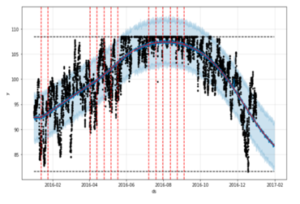
Figure 5: Forecast Plot with Prophet Built-in Method.

Observing the weekly plot provide by Prophet in Figure 6, we can conclude that the usage of electricity consumption in the building increased on weekdays following the function of the building as an office. Also, through advance analysis, we can see daily electricity usage in Figure 7 decreases at 8 p.m. and increases at 2 a.m. And the annual trend in Figure 8 shows energy usage increases in the mid-season and decreases in the late season.

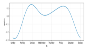
Figure 6: Weekly Plot of Energy Consumptions.

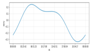
Figure 7: Daily Plot of Energy Consumptions.

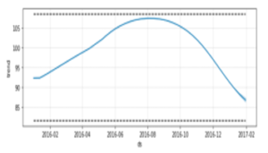
Figure 8: An Overview Plot of Energy Consumptions by Date.

4.2. Evaluation

We could investigate the trend of cross-validation errors for the next two months’ predictions in Figure 9. The blue line shows the RMSE, where the mean takes over a rolling window of the dots. We realize that errors below 5 points are typical for predictions one month into the future and that errors increase up to around 8 points for predictions two months into the future.

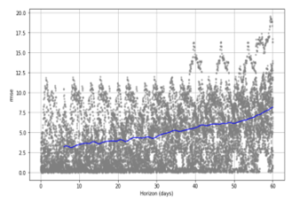
Figure 9: Cross Validation Visually Over Time.

Another experiment had conducted to further evaluate the Prophet’s performance with another well-known time series algorithm, LSTM. For  LSTM  training model configuration, we use two hidden layers, with each consisting of  50 LSTM units, dropout 0.25, batch size 32, and a sliding window of 720 as the accumulated number of hours in one month. And weather dimensions applied previously in the normalization process were used as inputs in the LSTM model.

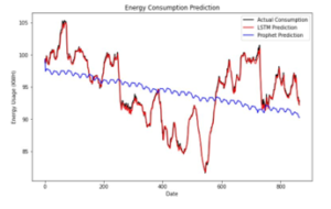Figure 10: Prophet, LSTM Prediction and Actual Comparison.

Looking at the results on the graph in Figure 10, it appears prophet performs well in fitting data without overfitting. On the other hand, LSTM tends to shows easily overfitting results with RMSE around 0.005 points and training execution time around 330 s. Meanwhile, Prophet with just one-dimensional feature input showed a short training time of 20 s, 15 times faster than LSTM. Comprehensively LSTM still needs to apply an approach to minimize overfitting.  Adding more data to LSTM maybe become the solution to have reasonable predictability results.

Cross-validation may be used for tuning hyperparameters of the model, as can be seen in Figure 11. Here parameters are evaluated on RMSE averaged over a 30-day horizon. However, different performance metrics may be acceptable for various problems. In this scenario, the changepoint prior scale is specified within [0.001; 0.01; 0.1; 0.5], while the seasonality prior scale within [0.01, 0.1, 1. 10]. Seeing the result, whereas an increase of changepoint ratio may offer minimum RMSE, nevertheless, it tends to form the model overfitting after all.

Figure 11: Hyperparameter Tuning on Prophet Parameters.

5. Conclusion

With the rapid advancement of machine learning-based techniques, especially deep learning algorithms, the Prophet method is gaining popularity as alternatives way among researchers across diverse disciplines. The objective of this study was to improve the baseline model by introducing the implementation of prophet methods with its practical advantages combine with weather normalization method SDE U/L. Furthermore, we would highlight some of its ability within this experiment in addressing a variety of external factors that affect electricity consumption, such as modeling holiday effects, custom seasonalities, and additional regressor. As a result, SDE U/L – Prophet models could considered successfully predicted values without overfitting in the 30-day forecast with maximum RMSE around 5 points. In advance, more data will make predictions give better results. In the future, the Prophet can be a leading solution that offers practically insightful, flexibility, accuracy, speed, and simplicity for many non-technical users in various time series cases.

We hope that this study result could be a consideration for the researcher by using Prophet methods in various time series cases, as many advantages that Prophet have compared to other time series prediction methods. And especially for practitioners to be more efficient in choosing the best energy-saving based on the prediction analysis result of the energy savings method used. So that in the future practitioner does not have to wait until months to evaluate the final results before further modification considering the many costs incurred in the method selection process. This provides a useful tool for analysts to gain insight into their forecasting problem, besides just producing a prediction.

1. Y. Ji et al., “Hybrid ventilation for low energy building design in south China. Building and Environment, 44(11), 2245-2255, 2009.
2. Z. Romani et al., “Metamodeling the heating and cooling energy needs and simultaneous building envelope optimization for low energy building design in Morocco. Energy and Buildings, 102, 139-148, 2015.
3. Y. Zhang et al., “A new approach, based on the inverse problem and variation method, for solving building energy and environment problems: preliminary study and illustrative examples. Building and Environment, 91, 204-218, 2015.
4. I. Choi et al., “Energy consumption characteristics of high-rise apartment buildings according to building shape and mixed-use development. Energy and Buildings, 46, 123-131, 2012.
5. S. Singaravel et al., “Component-based machine learning modelling approach for design stage building energy prediction: weather conditions and size. In Proceedings of the 15th IBPSA conference, 2617-2626, 2017.
6. E. Elkind, “Powering the Savings: How California Can Tap the Energy Efficiency Potential in Existing Commercial Buildings, 2016.
7. F. Rodrigues et al., “The daily and hourly energy consumption and load forecasting using artificial neural network method: a case study using a set of 93 households in Portugal. Energy Procedia, 62, 220-229, 2014.
8. R. Bonetto et al., “Machine Learning Approaches to Energy Consumption Forecasting in Households, 2017. https://arxiv.org/abs/1706.09648
9. I. Yenidoğan et al., “Bitcoin Forecasting Using ARIMA and PROPHET. In 2018 3rd International Conference on Computer Science and Engineering, 621-624, 2018.
10. H. Aguilera et al., “Towards flexible groundwater-level prediction for adaptive water management: using Facebook’s Prophet forecasting approach. Hydrological Sciences Journal, 64(12), 1504-1518, 2019.
11. C. Mi et al., “Real-time Recognition of Smartphone User Behavior Based on Prophet Algorithms, 2019. https://arxiv.org/abs/1909.08997
12. Z. Yu et al., “A systematic procedure to study the influence of occupant behavior on building energy consumption. Energy and buildings, 43(6), 1409-1417, 2019.
13. M. Ghajarkhosravi et al., “Energy benchmarking analysis of multi-unit residential buildings (MURBs) in Toronto, Canada. Journal of Building Engineering, 27, 100981, 2020.
14. R. Zmeureanu, “A new method for evaluating the normalized energy consumption in office buildings. Energy, 17(3), 235-246, 1992.
15. S. Beheshti et al., “Structure dependent weather normalization. Energy Science & Engineering, 7(2), 338-353, 2019.
16. S.N. Wood, ” Generalized additive models: an introduction with R. Chapman and Hall/CRC, 2017.
17. A.S. Weigend, “Time series prediction: forecasting the future and understanding the past, Routledge, 2018.
18. K. Larsen, “GAM: the predictive modeling silver bullet. Multithreaded. Stitch Fix, 30, 2015.
19. S.J. Taylor et al., “Forecasting at scale. The American Statistician, 72(1), 37-45, 2018.
20. K. Gajowniczek, “Short term electricity forecasting using individual smart meter data. Procedia Computer Science, 35, 589-597, 2014.
21. L. Wang et al., “Adaptive learning based data-driven models for predicting hourly building energy use. Energy and Buildings, 159, 454-461, 2018.
22. Ashrae, ASHRAE – Great Energy Predictor III, Version 1. Retrieved January 25, 2020. https://www.kaggle.com/c/ashrae-energy-prediction/data.
23. P.J. Fabri, “Measurement and Analysis in Transforming Healthcare Delivery. Springer, 2016.

(Click Here)

(Click Here)