1. Introduction

Digital signal processing is one of the most pressing areas of science and technology today, which is developing from a practical point of view. The correct choice of mathematical apparatus in the digital processing of signals leads to a high degree of accuracy in making the right decisions by experts in the field. As an example, we can say that in medicine and geophysics accuracy is very important [1]. In medicine, accuracy plays an important role in such processes as determining the current condition of a patient brought to the hospital in a critical condition, determining the type of disease, clarify  the degree of the disease. We know that in the field of geophysics, too, a large amount of money is spent on the extraction of mineral resources, so accuracy is important in confirm the location of minerals [2].That is, according to the anomalous changes in the geophysical signal, it is possible to make predictions for the analysis  the subsequent developmental activity of the object under study. Usually, as a result of forecasting, it is possible to predict such information as the location of the most accumulated minerals, the amount of their reserves in advance. As information can be used anomalous changes in the electromagnetic, gravitational fields of the earth, anomalous changes in the ionosphere, seismic noise, various acoustic vibrations.

Today, scientists are exploring new ways to process these signals using a variety of mathematical models and algorithms [3]. One of these methods is to recover the signals received in tabular form using local interpolation spline functions [4]. This is because the accuracy level of spline functions is higher than that of classical interpolation polynomials. And the algorithms derived from them require less computation [5]. Existing classical interpolation models, their application in signal recovery and digital processing algorithms are performed depending on the node points [6], [7]. The construction of classical interpolation polynomials is based on the idea of replacing functions with that are closer to it, in a sense, and simpler in structure [8], [9]. In this case, a large number of node points are required to obtain a high degree of convergence of these models [10], [11]. In the case of node points, the order of the system equations formed in the construction of the model under consideration increases, and the process of solving this system of equations becomes more complicated, which does not ensure a high level of accuracy of the model.

In order to solve this problem, in the article, the process of digital processing of signals was carried out using high-precision spline models. The increase in the degree of convergence of the models under consideration does not depend on the increase in the order of the system of equations [12], [13].

That is, in the construction of the spline function considered in this work, the following node points are constructed on the basis of  in the  interval  local interpolated cubic spline.

That is, the spline function divides the [a, b] interval into n parts and builds a spline function in a single interval (Figure 1).

To construct a spline function, the interval [a, b] is divided into n parts, and the spline function is constructed in a single interval [14].

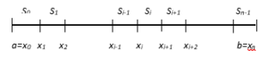
Figure 1: A view of the spaces where the cubic spline is built.

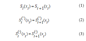
If conditions (1), (2) and (3) are met, the spline function defect is called a spline function that fully meets the actual level of demand, which is equal to 1.

The following is a study of cubic spline functions with high accuracy in digital processing of signals [15]-17].

2. Build cubic spline functions

In digital signal processing, cubic spline functions are a high-precision mathematical apparatus.

We know that the  corresponding to the function, the function passing through the node points, is called the interpolation cubic spline and meets the following conditions [1],[9],[10]:

• function third-degree polynomial in each  interval;
• The first and second-order derivatives of the function must be continuous in the interval [a, b];

The last condition is called the interpolation condition, and the function that satisfies the three conditions is called the interpolation cubic spline.

2.1.  Build a cubic spline function based on basic functions

Let us be given the following function.

Assume that the node points on the  axis are defined in steps h as follows [12].

In turn,  and are also calculated sequentially as above.

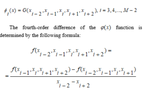
After some simplification, the calculation formula for the fourth-order subtraction difference of the  function will look like this:

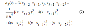
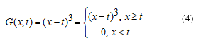
Based on the features discussed above, the following forms the basis in the space of tertiary splines

Let’s look at the features.

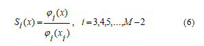
This function forms the basis in the space of cubic splines and has the following features:

1) Smoothness

The values of the function at the  node points are given .

Consider the following function.

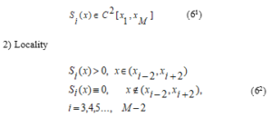
the local condition is required.

In that case, the values at the node point of the function based on the localization condition are as follows.

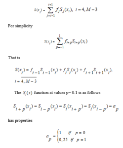
That is, at p = 0

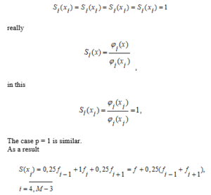
As a result

We now express the  through the , for which we spread them to the Taylor series

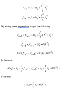
We will have .

The smoother the function, the closer it is to  in calculations.

And the spline function is close to the at the node points then we find the next approximate function

In that case

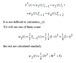
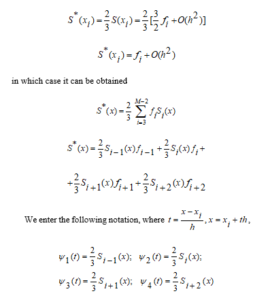
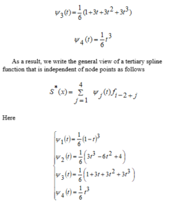
As a result, we write the general view of a tertiary spline function that is independent of node points as follows

2.2. Local interpolation cubic spline function based on Ryabenky operator

If the function is smooth enough, then it is advisable to approximate this function with spline functions. The use of third degree Given the extreme nature of the spline function with a high approximation accuracy, a third-order Ryabenky spline can be used to approximate the function, which approximates better than classical interpolation polynomials [10].

The  function belongs to the class of continuous functions up to the , q order derivative.

Where q> 0 is the fixed number. Let the values of the function be given at nodes of equal spacing

In Ryabenky’s article, a 2p+1 level  spline function with defect p+1 was constructed based on the  values of the  function. For the  error in the one-dimensional case (up to the derivative of order r < q), the following is appropriate.

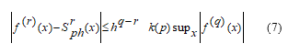
Where k(p) is not variable, it only depends on p.

For the optional p, the  spline can be written to see the exact appearance of the  function via  values. It is therefore very convenient to apply in various fields. This spline function can also be approximated in C[a,b] to the advantage of the Hermit spline.

In the works of S.L. Sobolev the following Ryabenky operator is given for the function in the  interval [14].

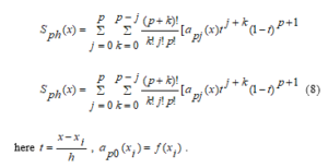
The spline function given in (8) is a 2p+1 level spline with a defect defect p+1, which in general gives a local third-order interpolation spline of the special case Ryabenky given p = 1.

When p= 1, a local cubic spline is formed

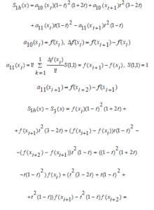
This function in the  interval (9) can be called the “Ryabenky” cubic spline function.

2.3. Building of a local interpolation cubic spline function

Divide the  interval into n equal parts

We construct the local interpolation cubic spline model under consideration using a linear combination of two  and   parabolas in the   interval [9],[13].

We have the following four points  to build a  spline in the  range.

It should be noted that in this method, four points are of course used to construct the interpolation cubic spline model (Figure 2).

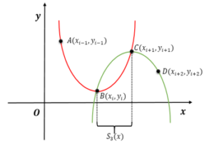
Figure 2: A view of the  local cubic spline construction range.

Using the interpolation condition to construct the following  parabola passing through the points , we construct the following system of equations [13], [18]:

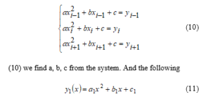
parabola will be formed.

We construct the following system of equations to construct the second  parabola passing through the  points as above:

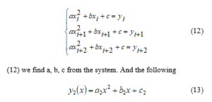
parabola will be formed.

We perform the replacement to make it easier to estimate the error here .

To determine the , we construct equations (16):

where are found

The system of equations (17) and (18) is formed after some simplification of the interpolation conditions of the first  and the second  at the  node point of the spline

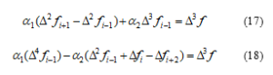
here  is the difference of operators.

If we say that the system of equations (16) – (18) is solved by  ,

Then

Spline will have 1 defect. But coefficients are complex rational functions. Therefore, such splines are inconvenient for digital processing of signals.

If we say , then  These values satisfy equations (16) – (17) but do not satisfy equation (18)

The defect of the interpolation spline in the   interval will be 2 [1],[13].

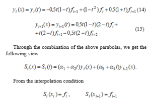
We will add these following formulas

Substituting the expressions (14) and (15) for the and given in (19), we obtain the view (20) for the  interval.

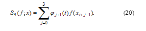
Based on the theory of splines, this function in the  interval (20) can be called a local interpolation cubic spline function.

3. Approximation of functions using local cubic splines

The graph of the local interpolation cubic spline function generated in Section 2 was compared with the graph of the Ryabenky local cubic spline function and the graph of the Grebennikov local cubic spline function.

Let us compare the approximation of these three local cubic splines with the given function .

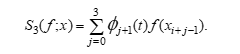
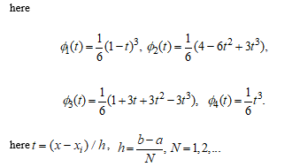
The local interpolation cubic spline function we propose has the appearance in у  cross section as studied in Section 2.3:

We then define this spline function with for convenience.

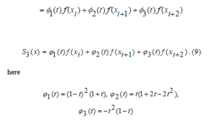
The second is the Ryabenky local cubic spline function and has the following appearance in у  cross section:

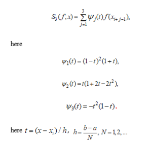
We define the Ryabenky local cubic spline function by

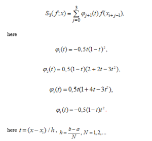
The third spline is the Grebennikov local cubic spline function, which has the following appearance in the cross section:

We define the Grebennikov local cubic spline function as . In the examples, without losing generality, we only look at the situation when there is .

In this case, we consider the approximation of several functions in  and graphs with three cubic splines (Figures 3,4,5 and 6):

1. In the case of (examples given in Fig. 3)

As can be seen from the graph of the first example, the spline graph overlaps with the function graph, while the  and  spline graphs do not overlap.

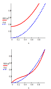
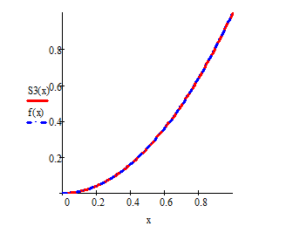
Figure 3: Results of approximation of the function with three cubic splines.

2. In the case of (examples given in Fig. 4)

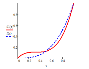
Figure 4: Results of approximation of the  function with three cubic splines.

3. In the case of

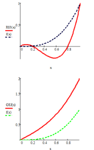
Figure 5: Results of approximation of the function with three cubic splines

4. In the case of

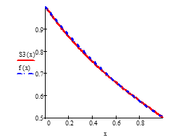
Figure 6: Results of approximation of the function with three cubic splines

Examples 1,2,3 and 4 show that the spline function graph approximates the function graph better than the and spline function graphs.

4. Digital processing of gastroenterological signals based on developed algorithms

Using the cubic spline models considered, the restoration of the gastroenterological signal given in Table 1 was considered. Based on the above sequence, a tertiary spline construction program was developed in the MATLAB software environment and used in signal processing (Figure 7). The algorithm of this program is shown in Figure 8.

Table 1: Values of the gastroenterological signal

№	Time, s	Amplitude	№	Time, s	Amplitude
1.	1	0.051	26.	26	0.085
2.	2	0.056	27.	27	0.058
3.	3	0.049	28.	28	0.021
4.	4	0.069	29.	29	0.004
5.	5	0.097	30.	30	0.037
6.	6	0.132	31.	31	0.036
7.	7	0.066	32.	32	0.099
8.	8	0.118	33.	33	0.094
9.	9	0.080	34.	34	0.075
10.	10	0.090	35.	35	0.064
11.	11	0.072	36.	36	0.034
12.	12	0.043	37.	37	0.067
13.	13	0.112	38.	38	0.045
14.	14	0.128	39.	39	0.063
15.	15	0.109	40.	40	0.069
16.	16	0.056	41.	41	0.069
17.	17	0.121	42.	42	0.097
18.	18	0.091	43.	43	0.077
19.	19	0.138	44.	44	0.066
20.	20	0.142	45.	45	0.093
21.	21	0.119	46.	46	0.061
22.	22	0.053	47.	47	0.048
23.	23	0.074	48.	48	0.085
24.	24	0.107	49.	49	0.113
25.	25	0.107	50.	50	0.078

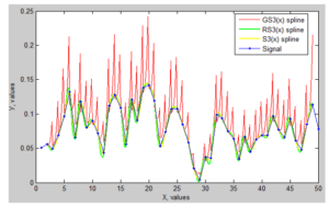
Figure 7. Results of gastroenterological signal recovery

Table 2: Error results in the process of digital processing of the gastroenterological signal

2	0,056	0,0562	0,056	0,056	0,0002	0	0
2.1	0,0553	0,0589	0,0551	0,0557	0,0036	0,0002	0,0004
2.2	0,0546	0,0632	0,0537	0,0549	0,0086	0,0009	0,0003
2.3	0,0539	0,0694	0,0522	0,0539	0,0155	0,0017	0
2.4	0,0532	0,0778	0,0506	0,0528	0,0246	0,0026	0,0004
2.5	0,0525	0,0887	0,0491	0,0516	0,0362	0,0034	0,0009
2.6	0,0518	0,0535	0,0479	0,0504	0,0017	0,0039	0,0014
2.7	0,0511	0,0544	0,0471	0,0495	0,0033	0,004	0,0016
2.8	0,0504	0,0559	0,0469	0,0489	0,0055	0,0035	0,0015
2.9	0,0497	0,0584	0,0475	0,0487	0,0087	0,0022	0,001
3	0,049	0,0625	0,049	0,049	0,0135	0	0
3.1	0,051	0,0684	0,0509	0,0499	0,0174	0,0001	0,0011
3.2	0,053	0,0765	0,0527	0,0511	0,0235	0,0003	0,0019
3.3	0,055	0,0872	0,0545	0,0528	0,0322	0,0005	0,0022
3.4	0,057	0,101	0,0562	0,0547	0,044	0,0008	0,0023
3.5	0,059	0,1183	0,058	0,0568	0,0593	0,001	0,0022
3.6	0,061	0,0703	0,0598	0,0591	0,0093	0,0012	0,0019
3.7	0,063	0,0729	0,0618	0,0616	0,0099	0,0012	0,0014
3.8	0,065	0,0761	0,064	0,0641	0,0111	0,001	0,0009
3.9	0,067	0,0805	0,0664	0,0666	0,0135	0,0006	0,0004
4	0,069	0,0868	0,069	0,069	0,0178	0	0
					0,0593	0,0040	0,0023

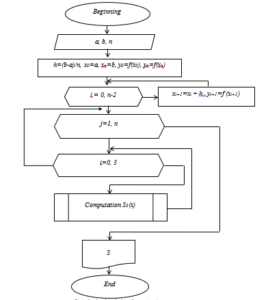
Figure 8: Algorithm of cubic spline construction program.

here, a and b are the limits of a given interval, n is the number of intervals of the interval.

5. Conclusion

In this article, spline functions with a high degree of accuracy in digital processing of signals which are Grebennikov cubic spline, the Ryabenky cubic spline, and the local interpolation cubic spline functions that we proposed.

The construction details selected cubic spline-functions in the equally distributed nets were given, and initially the processes of approximation functions were carried out.

Using selected cubic spline models, the gastroentrological signal was digitally processed and errors were evaluated.

According to results of approximation function using local cubic splines presented in Section 2, as well as the error results in Table 2 obtained from digital processing of the gastroenterological signal, it was found that the local interpolation cubic spline accuracy was high which .we proposed

It can be seen that the application of the mathematical model of the local interpolation cubic spline function we have considered in medicine, in geophysics, and in many areas where the level of accuracy is important in digital processing and recovery of signals leads to effective results.

1. Z. Xakimjon, A. Bunyod, “Biomedical signals interpolation spline models,” in International Conference on Information Science and Communications Technologies: Applications, Trends and Opportunities, ICISCT 2019, 2019, doi:10.1109/ICISCT47635.2019.9011926.
2. J. Rajeswari, M. Jagannath, Advances in biomedical signal and image processing – A systematic review, Informatics in Medicine Unlocked, 8, 2017, doi:10.1016/j.imu.2017.04.002.
3. A. Subasi, Biomedical Signal Processing Techniques, 2019, doi:10.1016/b978-0-12-817444-9.00003-9.
4. S. Patidar, T. Panigrahi, “Detection of epileptic seizure using Kraskov entropy applied on tunable-Q wavelet transform of EEG signals,” Biomedical Signal Processing and Control, 34, 2017, doi:10.1016/j.bspc.2017.01.001.
5. M. Unser, “Splines: A Perfect Fit for Signal and Image Processing,” IEEE Signal Processing Magazine, 16(6), 1999, doi:10.1109/79.799930.
6. K. Usman, M. Ramdhani, “Comparison of Classical Interpolation Methods and Compressive Sensing for Missing Data Reconstruction,” in Proceedings – 2019 IEEE International Conference on Signals and Systems, ICSigSys 2019, 2019, doi:10.1109/ICSIGSYS.2019.8811057.
7. D. Singh, M. Singh, Z. Hakimjon, Geophysical application for splines, 2019, doi:10.1007/978-981-13-2239-6_7.
8. G. Lindfield, J. Penny, Numerical methods: Using MATLAB, 2018, doi:10.1016/C2016-0-00395-9.
9. A.I. Grebennikov, “Isogeometric approximation of functions of one variable,” USSR Computational Mathematics and Mathematical Physics, 22(6), 1982, doi:10.1016/0041-5553(82)90095-7.
10. D. Singh, M. Singh, Z. Hakimjon, B-Spline approximation for polynomial splines, 2019, doi:10.1007/978-981-13-2239-6_2.
11. M. Singh, H. Zaynidinov, M. Zaynutdinova, D. Singh, “Bi-cubic spline based temperature measurement in the thermal field for navigation and time system,” Journal of Applied Science and Engineering, 22(3), 2019, doi:10.6180/jase.201909_22(3).0019.
12. H.N. Zayniddinov, O.U. Mallayev, “Paralleling of calculations and vectorization of processes in digital treatment of seismic signals by cubic spline,” in IOP Conference Series: Materials Science and Engineering, 2019, doi:10.1088/1757-899X/537/3/032002.
13. H. Zaynidinov, M. Zaynutdinova, E. Nazirova, “Digital processing of two-dimensional signals in the basis of Haar wavelets,” in ACM International Conference Proceeding Series, 2018, doi:10.1145/3274005.3274023.
14. S.L. Sobolev, Selected Works of S.L. Sobolev, Springer US, Boston, MA, 2006, doi:10.1007/978-0-387-34149-1.
15. Y. Kim, G. Lee, S. Park, B. Kim, J.O. Park, J.H. Cho, “Pressure monitoring system in gastro-intestinal tract,” in Proceedings – IEEE International Conference on Robotics and Automation, 2005, doi:10.1109/ROBOT.2005.1570298.
16. B.H. Jansen, “ANALYSIS OF BIOMEDICAL SIGNALS BY MEANS OF LINEAR MODELING.,” Critical Reviews in Biomedical Engineering, 12(4), 1985.
17. H. Zaynidinov, J. Juraev, U. Juraev, “Digital image processing with two-dimensional haar wavelets,” International Journal of Advanced Trends in Computer Science and Engineering, 9(3), 2020, doi:10.30534/ijatcse/2020/38932020.
18. D. Singh, M. Singh, Z. Hakimjon, Parabolic Splines based One-Dimensional Polynomial, 2019, doi:10.1007/978-981-13-2239-6_1.

(Click Here)

(Click Here)