1. Introduction

Electrical Impedance Tomography (EIT) is useful for visualising the conductivity distributions of an imaged space. Due to its non-intrusiveness, low cost and versatility, EIT has been widely used in medical [1] and industrial [2] applications. Recently, EIT is gaining more attention in industrial applications as it provides intuitions and insights to the reaction and dynamic of the process, as well as useful information of flow characteristic in a pipeline or process vessel. However, EIT imaging suffers from relatively low spatial resolution, especially towards the centre of the imaged space, which is ultimately impacting the quality of the reconstructed images. This is due to the ill-posed nature of the EIT problem [3]. As a result, numerous efforts have been made to further understand this problem and explore ways to improve spatial resolution in EIT imaging.

In an EIT system, the planar arrangement is a commonly employed electrode configuration, where electrodes are mounted in an equally spaced manner, on the perimeter of the process tank or vessel, and the centre of electrodes are aligned on a defined height. In industrial applications, an effective electrode configuration system greatly depends on the vessel or tank size. The criteria of the electrode configuration include the plane spacing between electrode planes and the number and size of electrodes. So far, there is no past work that studied plane spacing of the multiple electrode planes in EIT applications systematically. Instead, the past publications are more focus on the electrode parameters, such as size and number of electrodes, in medical and industrial applications.

In [4], the authors investigated the optimal distance of the multiple sensor plane using a 3D EIT imaging technique based on simulation and experimental study. The investigation showed that the quality of the reconstructed images was accessed based on the correlation coefficient and the relative error. The results showed that 3.5 cm plane spacing between electrode planes, for a model with a diameter of 16 cm and a height of 21.5 cm, produced the highest value in correlation and achieved the lowest values in the relative errors as well as provided optimal performance in the distribution tests. In [5], the authors investigated the performance of drive and measurement electrode patterns using various plane spacing between electrode planes. The results highlighted that the Signal to Error (SNR) decreases as the spacing between two electrode planes decreases, regardless of the transverse and longitudinal current patterns applied. The transverse current patterns provided a better resolution than longitudinal current patterns but were more susceptible to noise and error, leading to poorer sensitivity in detecting impedance changes in the centre of imaged space. However, in industrial applications, the plane spacing between electrode planes may become a minor concern for the researchers.

Electrode parameters, such as size and number of electrodes, have been investigated in the past few decades. In [5], an experiment was carried out to examine the effect of the height of electrodes on the quality of reconstructed images. The findings indicated that the sensitivity or detectability of the EIT system reduced or remained the same as the height of electrodes was increased to twice the height of the imaged object or target. In [6], the authors investigated the optimum sized electrodes for Electrical Resistance Tomography (ERT). The findings highlighted that the optimum size of electrode coverage is 60% and 80% of the wall surface area of the model. In [7], [8], the authors investigated the electrode properties of ERT. They found that dot or point electrodes could eliminate the effect of contact impedance. Dot or point electrodes are more commonly applied in medical applications. However, it is impractical when implementing dot or point electrodes in industrial applications, as it is more costly to fabricate [9].

Electrodes used in applications are often in rectangular shape. This is not ideal, as narrow angles on the electrode corners result higher current densities in these areas. Circular electrodes are ideal for this purpose due to the uniformity of its shape [10]. However, forward solving requires discretisation of the model into tetrahedral elements in EIT. An accurate modelling of circular electrodes requires a large number of small elements to best represent the shape of electrodes, which results in an increased number of computational elements, and more importantly, these elements do not contribute to the representation of the imaged space. When the coarser mesh structure is used, the inaccurate representation of the shape of the electrode will occur and it leads to errors in forward and inverse solving. As a compromise, rectangular electrodes are often used.

In this paper, the influence of different plane spacing between electrode planes on EIT applications in industrial processes (e.g. pipeline flow and suspension monitoring, and mixing processes) on the quality of reconstructed images is studied. The main purpose of this investigation is to investigate a minimum requirement of space between electrode planes, such that information is not lost. This investigation was carried out through investigating the effect of different electrode configurations on imaging properties and reconstructed images. The rest of the paper consists of five (5) sections.  The model setup for various plane spacing between electrode planes is described in Section II. Section III discusses the findings obtained from the comparative studies on image properties. Section IV describes the experimental setup for image reconstruction, as well as its results. Finally, Section V provides the conclusion of this study.

2. Model Setup

In this work, a cylindrical model with a radius of 71.4 cm and a height of 80 cm is used. The dimensions of the model are chosen to be sufficiently big, such that it can accommodate a variety of different electrode configurations, including spacing between electrode planes, which is the main focus of the work presented in this paper.

The electrode configuration used for this work consists of 32 electrodes arranged in two planes. Each plane consists of 16 electrodes arranged equi-spaced on the periphery of the model. The electrodes are rectangular in shape, with the dimensions of 3 cm in width and 10 cm in height. In this study, the spacing between planes is set as 5 cm (the smallest gap), 10 cm, 15 cm, 20 cm, 25 cm and 30 cm (largest gap). A summary of the plane spacing between electrode planes and the height of the centre of the upper and lower electrode planes is provided in Table I.

Table 1: Plane Spacing Between Two Electrode Planes and its Center of Upper and Lower Electrode Plane

Number of electrodes per plane	Plane spacing between two electrode planes	Center of upper electrode plane (cm)	Center of lower electrode plane (cm)
16	5 cm	47.5	32.5
	10 cm	50.0	30.0
	15 cm	52.5	27.5
	20 cm	55.0	25.0
	25 cm	57.5	22.5
	30 cm	60.0	20.0

The work presented in this paper is simulated using Electrical Impedance Tomography and Diffuse Optical Tomography Reconstruction Software (EIDORS), which is an open-source toolkit available for MATLAB [11]. The discretisation of the models was done by applying the Finite Element Method (FEM) through Netgen [12]. The FEM models with various spacing between electrodes planes are as depicted in Figure 1. It is should be noted that the number of elements for each of the models is the same as they are based on the same cylindrical model. The work presented in this paper is through simulation as it is a more feasible option due to the requirement of using electrodes with different plane spacing.

• 5 cm plane spacing between electrode planes model
• 30 cm plane spacing between electrode planes model

Figure 1: Examples of FEM models with varying plane spacing between electrode planes.

All measurements were simulated using the adjacent current injection protocol, which produces N*(N-3) number of measurements, where N is the number of electrodes. In the case of two planes of 16-electrodes per plane model, 416 full-frame measurements were generated. Another set of measurement data were repeated to simulate by using another opposite current injection protocol, which produces N*(N-4) number of measurements. There are 384 full-frame measurements generated for a model with two planes of 16-electrodes per plane.

3. Experimental Results

3.1. Sensitivity Analysis

Sensitivity analysis provides information on the potential success of detecting any changes in conductivity in the imaged space. In the discretised model, each element has a sensitivity value for any measurement acquired, which makes up the sensitivity (Jacobian) matrix. For this comparative study, the maximum sensitivity for each discretised element for a full set of measurement, normalised to the volume of the element, is computed and compared, as shown in Figure 4 and Figure 5.

Figure 4: Sensitivity comparison for models with different plane spacing electrode planes at the off-electrode plane (the height is taken at 0.40 m from the bottom of the model) by applying the (a) adjacent strategy and (b) opposite strategy.

Figure 4(a) shows the comparison of maximum sensitivity magnitude for the models with different spacing between electrode planes across an off-electrode plane when applying adjacent current injection protocol. From Figure 4(a), it can be seen that there are insignificant differences, as the spacing between electrode planes increases, especially towards the centre of the imaged space. Similar results are observed using the opposite current injection strategy, as reflected in Figure 4(b). This may due to the planar measurement strategy used, whereby measurements are only taken on the plane where the current source and sink pairs are located.

• The model with 5 cm plane spacing between electrode planes
• The model with 30 cm plane spacing between electrode planes

Figure 5: Sensitivity comparison for the models both (a) 5 cm and (b) 30 cm plane spacing between electrode planes, respectively, at the off-electrode plane and on the electrode plane.

From Figure 5, sensitivity is higher for opposite strategy due to the current penetrating through the imaged space, as opposed to the adjacent strategy, where current flowing typically tends to be more confined nearer to the periphery of the model [13]. The other obvious observation is that the sensitivity is higher on the electrode plane in comparison to those obtained off-electrode plane. This is expected, as the current signal is stronger on the electrode plane compared to the off-electrode plane [14]. This observation is similar to a previous study [15], where it indicates that the possibility of detecting a change in conductivity reduces when further away from the electrode plane.

Comparing Figure 5(a) and Figure 5(b), it can be observed that when the space between electrode planes are smaller (5 cm), there are insignificant differences between sensitivity on- and off-electrode planes. This is likely to be due to the closeness of the locations of the two electrode planes. In comparisons, when the space between electrode planes is bigger (30 cm), there are noticeable differences between sensitivity on- and off-electrode planes. Although the EIT image reconstruction problem is often treated as a 2D problem, where images and data are captured on a specific plane, it is essentially a 3D problem.

3.2. Spatial Resolution Analysis

Spatial resolution analysis utilises information given in the resolution matrix, which contains the correlation between elements in a discretised model. In this analysis, the Full-Width Half-Maximum (FWHM) technique [16] is applied to investigate the spatial resolution of models with different spacing between electrode planes. The FWHM method applied in this paper is based on the technique, which was first proposed by [17] and later adopted by [18]. In spatial resolution analysis, the minimum distance between two point sources, which shares the same solution value in an image is measured. The same solution value shared is known as half the peak value. Spatial resolution for each point is computed and compared. The results are as shown in Figure 6 and Figure 7.

Figure 6 shows the spatial resolution comparing models with different spacing between electrode planes using both adjacent and opposite strategies. It is shown that the regions near the wall of the model, in general, have better resolution (low FWHM) in comparison with the area towards the centre of the model, which resulted in higher FWHM. This general trend obtained is consistent with the sensitivity analysis obtained in Figure 4(a) and Figure 4(b), where they indicate that sensitivity is lower in the centre of the model but is higher near the wall region of the model. With a higher possibility of detecting a change in conductivity, and thus it increases the chance of change detected to be reconstructed.

It is worth noting that unlike the sensitivity analysis, spatial resolutions do not show symmetry across the plane, and irregularities (i.e. peaks or valleys) are observed. One of the factors that affect spatial resolution is the size of the discretised element, and unlike sensitivity analysis, the computed spatial resolution for each discretised element is not normalized to the volume of the element, as it will provide misrepresentation on the visibility contrast.

From Figure 6(a), it can be observed that models with 5 and 10 cm plane spacing between electrode planes produced the worst resolution overall, especially in the centre region of the model. However, it is worth noticing that model with 20 cm plane spacing between electrode planes resulted in better spatial resolution in general. This finding is not anticipated as the sensitivity analyses are shown in Figure 4, where it indicates that there are insignificant differences in maximum sensitivity magnitude across the off-electrode plane, for both current injection strategies.

Referring to Figure 7, comparing spatial resolution for the on- and off-electrode planes, it is observed that there are insignificant differences in the resolution for an on-electrode plane, especially with the gap between the two electrode planes is small (5 cm). This result is consistent with the results observed in its corresponding comparative analysis, as shown in Figure 5. The spatial resolution analysis in Figure 7 also shows that the overall resolution is evenly matched for usable information which is available for image reconstruction.

Figure 6: Spatial resolution comparison for models with different plane spacing by applying adjacent strategy in (a) and opposite strategy in (b) at 0.40 m height from the base of the model.

It is interesting to see in Figure 7(a) that there is very little difference in spatial resolution when comparing spatial resolutions for the adjacent and opposite strategies. This is unexpected, as shown in Figure 5, where there is a distinguishable difference in sensitivity between the two different measurement strategies. One of the reasons is likely to be due to both strategies producing a similar amount of usable (stable) information for reconstruction, which resulted in the spatial resolution for these two strategies to be evenly matched.

4. Experimental Set-up

4.1. Experimental Set-Up

Measurements for image reconstruction are simulated using the EIDORS package [11], which is MATLAB-based. As mentioned earlier, this study is more feasible to be done in simulation, as laboratory validation requires a process tank that allows multiple settings for electrodes configurations. For validation, two test distributions are used for experiment and comparison.

• The model with 5 cm plane spacing between electrode planes
• The model with 30 cm plane spacing between electrode planes

Figure 7: Spatial resolution comparison for the models both (a) 5 cm and (b) 30 cm plane spacing between electrode planes, respectively, at the off-electrode plane and on the electrode plane.

Measurements are simulated using a finely discretised FEM model. The level of discretization is chosen to be significantly  higher than the discretized model used for forward and inverse solving, as it is intended to mimic a physical model. Two measurements are taken for each test distribution, for each electrode configuration, and each measurement strategy.

In this work, two test distributions are used for image reconstruction, as shown in Figure 8. The first test distribution consists of two cylinders, each with a radius of 12 cm. The conductivity of the background is 0.012 S/m (approximately the conductivity value of tap water). One of the cylinders has a higher conductivity than background conductivity, and the other is non-conducting. The arrangement of test objects is as shown in Figure 8(a). The second test distribution is similar to the first test distribution, with the addition of one conducting cylinder. The arrangement of test objects is as shown in Figure 8(b). All reconstructed images were obtained by applying the Non-Linear Gauss-Newton (NLGN) algorithm in inverse solving.

• True distribution with two cylindrical objects
• True distribution with four cylindrical objects

Figure 8: True distribution models with (a) two cylindrical objects, (b) four cylindrical objects and (c) four floating objects. The colour scale is applied, where yellow colour indicates the conducting object and blue colour indicates the non-conducting object.

4.2. Results and Discussions

The image reconstructions obtained from models with different spacing between electrode planes are shown in Figure 9 to Figure 12. The colour scale is maximised to show the best contrast. The reconstructed images are assessed and discussed based on the dimensions of the reconstructed objects and colour contrast of the reconstructed conductivity distribution.

Although sensitivity analyses indicated there are insignificant differences in the maximum sensitivity magnitude as the gap between electrode planes increases, this is not reflected in spatial resolution analysis and reconstructed images. When comparing the reconstructed images from Figure 9-12, it can be seen that there are visible differences in terms of shape and estimation of dimensions of the objects.

In Figures 9-12, it can be seen that the models with 5cm and 10 cm plane spacing between electrode planes generally produced the worst reconstruction images. The shape and the dimension of the cylindrical test objects are not reconstructed properly, especially towards the top and the bottom of the imaged space. There are also noticeable artefacts visible in the imaged space. The results are similar for experiments done using both the adjacent and opposite strategies.

• 5 cm plane spacing between electrode planes
• 10 cm plane spacing between electrode planes
• 15 cm plane spacing between electrode planes
• 20 cm plane spacing between electrode planes
• 25 cm plane spacing between electrode planes
• 30 cm plane spacing between electrode planes

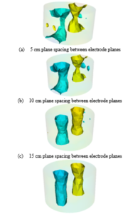
Figure 9: Reconstructed images comparison for models with various plane spacing (a)-(f) by applying the adjacent current protocol.

• 5 cm plane spacing between electrode planes
• 10 cm plane spacing between electrode planes
• 15 cm plane spacing between electrode planes
• 20 cm plane spacing between electrode planes
• 25 cm plane spacing between electrode planes
• 30 cm plane spacing between electrode planes

Figure 10: Reconstructed images comparison for models with various plane spacing (a)-(f) by applying the opposite current protocol.

• 5 cm plane spacing between electrode planes
• 10 cm plane spacing between electrode planes
• 15 cm plane spacing between electrode planes
• 20 cm plane spacing between electrode planes
• 25 cm plane spacing between electrode planes
• 30 cm plane spacing between electrode planes

Figure 11: Reconstructed images comparison for models with various plane spacing (a)-(f) by applying the adjacent current protocol.

• 5 cm plane spacing between electrode planes
• 10 cm plane spacing between electrode planes
• 15 cm plane spacing between electrode planes
• 20 cm plane spacing between electrode planes
• 25 cm plane spacing between electrode planes
• 30 cm plane spacing between electrode planes

Figure 12: Reconstructed images comparison for models with various plane spacing (a)-(f) by applying the opposite current protocol.

Models with 15 cm and 20 cm gaps generally produced better reconstructed images. With the exception of the reconstructed image using a test distribution with four cylindrical objects, the application of the adjacent strategy for the model with 20 cm gap, it can be seen in Figures 9-12 that the cylindrical test objects are reconstructed in the right configuration, with similar dimensions to the true distribution. There are also little to no artefacts visible in the imaged space.

For the widest gaps, namely the 25 cm and 30 cm electrode spacing models, the images reconstructed using the opposite strategy are better compared to those obtained using the adjacent strategy. The images obtained using the adjacent strategy has a significant amount of artefacts, and it is noticeable that the shape of the test objects are not reconstructed correctly where the gap of the electrodes are (i.e. space between electrode planes). It can be seen in Figures 9(e-f) and 11 (e-f) that the dimensions are overestimated in that space. In contrast, reconstructed images obtained using the opposite strategy turn out better, with the test objects shown to be cylindrical objects, and with less artefacts. This result is consistent with the results observed in the sensitivity analyses.

5. Conclusion

A summary of the results is tabulated in Table 2. This study is conducted through two methods: statistical method, through comparing sensitivity and spatial resolution of different models used; and through reconstructed images.

Table 2: Summarization of the results on image properties

Analysis	Best model	Worst model
Sensitivity Analysis	Results are inconclusive; Opposite strategy is better than adjacent strategy
Spatial Resolution Analysis	15 and 20 cm gap (both strategies)	5 and 10 cm gap (both strategies)
Reconstructed Images	15 and 20 cm gap (opposite strategy)	5 and 10 cm gap (both strategies)

From Table 2, it can be seen that the results obtained through spatial resolution analysis are reflected in the reconstructed images, where the best quality and worst quality images are reflective of the results obtained through spatial analysis. In this case, however, the sensitivity analysis results were inconclusive, as the sensitivity level in the centre region of the imaged space is indistinguishable.

It is worth noting that the results given in Table 2 are relative to the dimension of the model used for this study. When the model is scaled up or scaled down, an investigation similar to that carried out in this study should be conducted to ensure that the scaling effect does not deteriorate the quality of the reconstructed images.

Through this work, it is shown that it is important to investigate the spacing between electrode plane, to ensure that the information is not lost due to the inability to capture any changes that occur. It is impractical to have electrode planes close to each other, as it will result in a waste of resources. Therefore, a minimal distance ought to be set in order to ensure that any changes in conductivity can be measured and the information can be used to reconstruct and visualize the changes.

Conflict of Interest

The authors declare no conflict of interest.

Acknowledgment

The authors would like to express their gratitude to the financial support provided by the KPT-RACE (RACE0010-TK-2013) grant, KPT-FRGS (FRGS0425-TK-1/2015) grant and UMS-SGA (SGA0007-2019) grant for this work.

1. H. X. Wang, C. Wang, W. L. Yin, “Optimum design of the structure of the electrode for a medical EIT system,” Measurement Science and Technology, 12(8), 1020–1023, 2001. https://doi.org/10.1088/0957-0233/12/8/305
2. J. Nowakowski, E. Hammer, D. Sankowski, D. Styra, R. Wajman, R. Banasiak and A.Romanowski, “New concept of ECT/ERT/GRT tomography for multiphase flow measurements,” Automatyka (pó³- rocznik AGH), 14, 741-748, 2010.
3. W. Lionheart, N. Polydorides and A. Borsic, Part 1: The Reconstruction Problem, In Holder D. (ed) Electrical Impedance Tomography: Methods, History and Applications, Bristol, 3-64, 2005.
4. Z. Hao, S. Yue, B. Sun, and H. Wang, “Optimal distance of multi-plane sensor in three-dimensional electrical impedance tomography,” Computer Assisted Surgery, 22, 326–338, 2017.
5. J. Hope, F. Vanholsbeeck, and A. McDaid, “Drive and measurement electrode patterns for electrode impedance tomography (EIT) imaging of neural patterns activity in peripheral nerve,” Biomedical Physics and Engineering Express, 4(6), 2018. https://doi.org/10.1088/2057-1976/aadff3
6. J. C. Newell, Y. Peng, P. M. Edic, R. S. Blue, H. Jain, and R. T. Newell, “Effect of electrode size on impedance images of two-and three-dimensional objects,” in 1998 IEEE Transactions on Biomedical Engineering, 45(4), 531–534, 1998. https://doi.org/10.1109/10.664209
7. P. A. T. Pinheiro, W. W. Loh, F. J. Dickin, “Optimal sized electrodes for electrical resistance tomography,” Electronics Letters, 34(1), 69-70, 1998. https://doi.org/10.1049/el:19980092
8. F. Dickin, M. Wang, “Electrical resistance tomography for process applications,” Measurement Science and Technology, 7(3), 247–260, 1996. https://doi.org/ 10.1109/10.664209
9. L. D. Suits, T. Sheahan, J. Lee, J. Santamarina, “Electrical Resistivity Tomography in cylindrical Cells—Guidelines for hardware pre-design,” Geotechnical Testing Journal, 33, 2010. https://doi.org/10.1520/GTJ102366.
10. M. Hanke, B. Harrach and N. Hyvonen,“ Justification of Point Electrode Models in Electrical Impedance Tomography,” Mathematical Models and Methods in Applied Sciences, 21(06), 1395–1413, 2011. https://doi.org/10.1142/S0218202511005362
11. K. S. Cheng, D. Isaacson, J.C. Newell, D.G. Gisser,“ Electrode models for electric current computed tomography,” in 1989 IEEE Trans. Biomed Engr., 36, 918–924, 1989.
12. N. Polydorides, W.R.B. Lionheart, “A Matlab toolkit for three-dimensional electrical impedance tomography: a contribution to the Electrical Impedance and Diffuse Optical Reconstruction Software project,” Meas. Sci. Technol., 13, 1871–1883, 2002.
13. J. Schoberl, Netgen: Automatic Mesh Generator, 2008.
14. P. O. Gaggero, “Miniaturization and distinguishability limits of electrical impedance tomography for biomedical application”, Ph. D Thesis, University of Neuchatel, 2011.
15. P. Metheral, D. C. Barber, R. H. Smallwood, “Three-dimensional electrical impedance tomography,” 380, 509-5012, 1996. https://doi.org/https://doi.org/10.1038/380509a0
16. J.L. Wheeler, W. Wang, M. Tang, “Á comparison of methods for measurement of spatial resolution in two-dimensional circular EIT images,” Physiol. Meas., 23, 169-175, 2002. https://doi.org/10.1088/0967-3334/23/1/316
17. S.C. Murphy, “Ad hoc electrode arrangement for electrical tomography,” Ph. D Thesis, University of Manchester, United Kingdom, 2008.
18. W. Menke, Geophysical Data Analysis: Discrete Inverse Theory (Rev. Ed), Academic Press: San Diego, 1989.

(Click Here)

(Click Here)