1. Introduction

This paper is an extension of the work originally presented in the 2019 IEEE International Conference on Artificial Intelligence and Computer Applications [1], where a novel mutating Particle swarm optimization (MuPSO) based solution was proposed for analyzing the inverse kinematic problem of multi-degree-of-freedom robot manipulator. It was observed that the basic parameters of the Particle swarm optimization (PSO) algorithm are incapable of analyzing robot optimization problems, and it was established that the PSO parameters need to be modified for robot analysis. Further investigations were published in [2] where various parameters were used to analyse the inverse kinematic problem of four popular robot configurations and a new range of parameters for solving robot optimization problems was established, thereby an optimized mutating PSO algorithm for robot analysis was developed. If the algorithm runs into stagnation while solving a robot optimization problem, the mutation function is used to generate a completely new swarm and all the information regarding the previous swarm is lost. It is keen to note that if a particle from the previous swarm is retained, that particle becomes the global best particle for the new swarm, making the entire swarm converge again at the previous solution. It was observed that it would be beneficial to save previously non-dominated solutions in an archive for future reference. This work therefore seeks to further modify the mutating PSO algorithm by implementing it with an archived elite learning system, and using the new eMuPSO algorithm for dynamic parameter estimation of a 6 Degree-of-freedom (DOF) industrial manipulator and finally compare the improved algorithm with other state of the art algorithms in analyzing 36 benchmark functions. The rest of the paper is structured as follows; section 2 presents previous literature, section 3 introduces the new Mutating PSO algorithm, section 4 presents the results of parameter estimation of robot manipulators, and compares the new PSO algorithm with state of the art swarm-based algorithms on thirty-six benchmark functions and finally section 5 concludes the findings.

2. Literature

In industrial robotics, a dynamic model determines the actuator force required to achieve the desired joint configuration, coupling effects and non-linearity of the system introduces dynamic uncertainties. These errors degrade the robot’s performance. Therefore, re-calibrating robot parameters are necessary for efficient robot analysis and control, that can only be achieved experimentally. In dynamic model estimation, obtaining experimental data requires that firstly, a linearized model of the robot manipulator is developed, then a trajectory that excites the robot’s rigid body dynamics is developed, afterwards input torque and output joint configuration data is experimentally obtained and finally the dynamic parameters are estimated. The accuracy of the estimation method is largely dependent on the chosen trajectory and measuring accuracy. The actuator torque can be measured from input electric currents while optic encoders are incorporated for measuring joint output conditions. The recent improvement in technology makes available encoders and reduction gears that are capable of preventing cumulative errors and minimizing gearbox backlash. Therefore, carefully selecting an exciting trajectory is paramount in dynamic model estimation. Reference [3] observed that the excitation trajectory can be optimized by minimizing the condition number of the observation matrix. The observation matrix is a function of only the joint variables; it enables the solution of nonlinear systems to be presented as linear. The condition number of the observation matrix is a measure of noise immunity, a value closer to unity results in a better signal to noise ratio (SNR). The presence of unidentifiable parameters results in a high condition number of the observation matrix. References [4, 5] proposed techniques for categorizing dynamic parameters into identifiable parameters, unidentifiable parameters, and identifiable parameters in linear combinations. These works suggested that eliminating unidentifiable parameters from the observation matrix enhances estimation accuracy. In [6, 7] a set of Minimal Linear Combinations (MLC) of identifiable dynamic parameters from the total amount of parameters to be identified was generated. Reference [8] proposed formulating the periodic Finite Fourier series (FFS) as an excitation trajectory. FFS inhibits noise interference, if the identification experiment is repeated several times, averaging the measured data in the time domain improves SNR. Reference [9] used a modified Fourier series (MFS), where the FFS is implemented on a circular trajectory in the Cartesian space such that the initial and final conditions of the joints are the same, permitting continuity in the optimization experiment without necessarily stopping and restarting the manipulator. The particle swarm optimization algorithm (PSO) is a stochastic metaheuristic swarm-based evolutionary algorithm (EA), each particle in the swarm is attracted towards the global best particle’s position and its personal best position denoted as (Gbest and Pbest). The velocity and position of canonical PSO are updated according to (1) and (2).

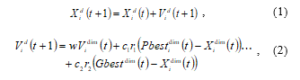
where i = 1, 2, 3…nPop denotes for the index of each particle, nPop is the swarm size, and dim = 1,2…dof denotes for the dimensionality of the solution space, dof is the degrees of freedom of the robot. V_i^dim and X_i^dim stand for the position and velocity vectors of the i^th particle, respectively. V_i^dim = [v_i¹, v_i², . . . , v_i^dof], X_i^dim = [x_i¹, x_i², . . . , x_i^dof ]. w is the inertia weight. c₁ and c₂ are cognitive and social learning coefficients. r₁ and r₂ are two uniformly distributed random numbers within the range of [0,1]. Over the years, PSO has undergone various modifications either to improve its internal dynamics (enhance convergence and exploitation characteristics) or to satisfy the requirement of a specific real-world optimization problem or both.

2.1. PSO with Improved Dynamics

An index based ring topology PSO was proposed by [10] for solving multimodal multi-objective optimization problems having more than one Pareto optimal solution corresponding to the same objective function. Reference [11] studied the impact of communication topology in PSO, the star topology (Gbest) where each particle communicates with every other particle, was found better in analyzing unimodal separable problems while the ring topology (LBest) where each particle communicates with only its two neighbor particles, is preferred for multimodal, non-separable and composite functions. The ring topology is more capable of jumping between optimum basins and it was also found to never converge at a local optimum, but with a considerably higher computational cost. Memetic algorithms (MA) are hybrid EAs that are a fusion of global and local search techniques. EAs are usually employed for global search while unconstrained optimizers are employed for local search. Adaptive MAs have been successfully combined with other EAs but not PSO, [12] proposed a co-evolutionary memetic PSO for solving multi-objective optimization problems. Feature selection (FS) is a combinatorial problem for large dimension data processing which requires large memory and high computational cost, [13] proposed a variable-length PSO for FS. The Proposed algorithm is flexible and simplifies large data analysis, and can jump out of local optima while narrowing the search space. The cooperative search strategy which prevents particle from being trapped in local optima was merged with PSO by [14] for unconstrained optimization, where cooperative multiple swarms were used to improve the convergence and efficiency of the canonical PSO.

2.2. Problem Oriented PSO

Medicine and medical healthcare are amongst the top beneficiaries of artificial intelligent swarm algorithms. Health care services are shifting from inpatients to outpatients. Reference [15] showed that accident and emergency centers in hospitals are currently being optimized to ensure 98% of patients get the required attention within 24 hours. The increasing demand for primary health care outlets has led to a requirement to optimize the operational efficiency of primary healthcare centers. Grouping the patients into an appropriate category optimizes time and manpower whereas patient no shows after grouping reduces operational efficiency of clinics.  In [16], using PSO to improve the accuracy of traditional clustering techniques was proposed for analyzing real-time patient attendance data and group them into clusters, while [15] compared PSO with opposition based learning and self-adaptive cohort intelligence for identifying significant features capable of predicting no shows. Gene selection from microarray data for cancer diagnosis and testing also involve large data sets and are computationally expensive, support vector machines algorithm is a fast and efficient classification model which requires its parameters tuned to satisfy specific problems. Reference [17] compared the performance of PSO-SVM and Memetic SVM for classification and feature selection of cancer cells. Alzheimer’s disease is a primary stage of dementia which is a type of memory disorder that affects the brain. The structural changes of the brain’s internal regions are the most commonly measured in diagnosing AD. Reference [18] compared the accuracy of PSO and other metaheuristic algorithms in segmenting the brain sub-regions. Air pollution is a major contributor to human mortality and a potential danger to the environment and ecological system [19]. Thermal power plants such as coal, petroleum, and natural gas are the main sources of air pollution, mercury contamination has been identified to be the most acute air pollutant produced by power plants [20]. In [21], a novel combination of modified genetic algorithm and the improved particle swarm optimization was proposed for minimizing the fuel cost of generating plants and emission simultaneously, by managing and controlling the integration of renewable energy and thermal power production, where an optimal generation plan for maximizing system efficiency can be achieved. Reference [22] proposed using an adaptive neuro-fuzzy inference system with PSO (ANFIS-PSO) for predicting mercury emission in power plants. Reference [23] sought to minimize the construction cost of reinforced concrete retaining walls (RCRW). These structures include bridges, railways, dams, etc., capable of withstanding the pressure resulting from the difference in level by an embankment, excavation, or natural processes. PSO was used to determine the optimum solution between popular techniques. In rural areas where the utility grid is unavailable, renewable energy is an attractive alternative for water pumping applications. The power-voltage curve of a photovoltaic cell was found to have multiple maximum power points under partial shading conditions, making the solar tracking mechanism unstable. In [24], the performance of PSO was compared with salp swarm algorithm for maximum power point tracking of solar panels. Electric motors are most popular for electrical-mechanical power conversion and employed in several industrial applications including robotics, because of their simplicity, durability, and low maintenance cost. They usually require a controller for high performance and efficiency. The electrical parameters of the electrical motor are very essential to design, performance assessment, and feasibility of the control technique, any difference in the actual motor parameters adversely affects the system performance. Reference [25] proposed using PSO for estimating the electrical parameters of induction motors.

3. Mutating PSO with Elite Archive Learning

The proposed PSO is equipped with a modified set of parameters and governing equations. The mutation function is used to generate a new swarm around the vicinity of the most promising particles when the algorithm runs into stagnation. The operation of the proposed mutating PSO with elite learning (eMuPSO) is divided into two, during the early stages, the algorithm searches the solution space for the minimum solution, then when it stagnates, elite solutions are being recalled from the archive and merged with the best solutions of the current run to generate a new population. The new population would be created either through Random or Gaussian mutation depending on the application. It was found that a mix of both was suitable for kinematic analysis while the Gaussian mutation was suitable for dynamic analysis.

3.1. Modified Parameters

It was established in [1] and [2] that the basic parameters of canonical PSO are not capable of ensuring converging solutions for robot optimization problems especially when the DOF is greater than three. The basic parameters of the mutating PSO were modified to satisfy the requirement for solving robot optimization problems. This was achieved by testing the performance of various PSO parameters on four popular robot configurations, and a relationship between the inertia weight and the social learning coefficient was derived. More details on modifying PSO parameters can be found in [2]. A non-linearly decreasing inertia weight is implemented with values between (2.1 – 0.6), the cognitive learning coefficient is constantly at 2.24, while the social learning coefficient is non-linearly increasing between (1.8 – 3.9). The equations for updating w and c2 are given in (3) and (4).

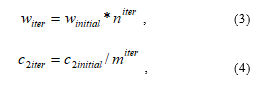
where iter is the iteration number, and n and m are coefficients. The coefficients n and m can be determined by setting iter to the maximum value. Robot configurations have complex dynamics described by highly coupled and non-linear, second-order differential equations, there are possibilities of numerous strong local minimizers in the solution space.

3.2. Mutation

In [26] it was shown that structural bias is a characteristic of swarm algorithms that tends to confine the algorithm to a region of the total search area. Mutation is a valid technique for overcoming such constraints. It was established in [2] that even the most intelligent swarm-based solutions are capable of running into stagnation, random mutation was used to push the algorithm out of stagnation and enhance convergence. The Gaussian mutation was used in [27] to improve swarm performance. Reference [28] also used a Gaussian mutation throw point strategy to redistribute the swarm at sparse positions. In the proposed algorithm, when the swarm stagnates at a local minimum solution, a Gaussian mutation is used to push the algorithm out of stagnation and redistribute the swarm to enhance unbiased coverage of the search space. The radius of the swarm is monitored according to (5). When the swarm radius becomes too small, it signifies that the swarm has lost diversity and might be stagnating, then the mutation function is initiated. The condition in (6) states that if there is no change in the swarm radius or when the change in the swarm radius is negligible, then the counter g increases sequentially otherwise the counter is reset to zero. A second condition in (7) terminates the algorithm when the minimum solution is achieved or the swarm is mutated when g is greater than a threshold value G.

Assuming there are k elite particles, the entire swarm population would be divided into k+1 parts and each k part would be replaced by off-springs of the k^th elite particle, while the k+1 part consists of particles generated from a random distribution, thereby maintaining diversity in the swarm. such that if x^dim is the dim^th dimension of the swarm, then all the elements in the dim^th dimension shall mutate according to (8).

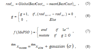
where rad is the radius of the swarm, iter refers to the current iteration, ^dimx_mutate and x_elite are the mutated off-spring and the elite solution in the dim^th dimension of the swarm, and σ is a variable between [0-1] multiplied by size of the search space.

3.3. Elite Archive

When the algorithm is searching for the best solution, the experiences of the best particle is transferred to the next iteration through the global best information, but at the beginning of subsequent generation or after mutation, all the information regarding the best particle from the previous generation is lost. This inspired the introduction of an archive where the experiences of the elite non-dominated solutions are saved and can be called in the future to enhance the search. Reference [29] applied a dynamic archive maintenance strategy to improve the diversity of solutions in multi-objective particle swarm optimization. In [30] an external archive was employed to preserve the non-dominated solutions visited by the particles to enable evolutionary search strategies to exchange useful information among them, and [31] used a grid-based approach for the archiving process and ε-dominance method to update the archive, which helps the algorithm to increase the diversity of solutions. Reference [32] used the cooperative archive to exploit the valuable information of the current swarm and archive. Information about the elite particles from dynamic sub swarms was used in [33] to improve the following sub-swarm, while [32] introduced a new velocity updating technique that explores the external archive of non-dominated solutions in the current swarm. In this article, an elite archive learning is used to refine the solution in the final stages of the algorithm. Elites from previous searches are saved as global elites, while elites of the current search are saved as local elites. When the algorithm stagnates, a combination of both elite vectors is used to generate a new population, and the global elites are updated with new solutions from the current local solutions

3.4. Robot Dynamics

Industrial robot manipulator

A 6 DOF industrial robot manipulator was analyzed, the structure of the robot manipulator is shown in Figure 1 and its D-H parameters are given in Table 1. A homogeneous transformation matrix describes the state (orientation and position coordinates) of a robot link with respect to the previous link in the Cartesian coordinate space and can be used to describe the state of the end-effector (tool) of the manipulator with respect to the base (global coordinate) frame. If all the joint parameters are known (D-H Parameters), the homogeneous matrix of each successive pair of frames for the forward and inverse directions can be obtained from (9). The robot manipulator’s end-effector coordinates would be a product of post multiplication as shown in (10).

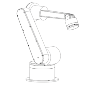
Figure 1: A 6 degree of freedom industrial robot manipulator

Table 1: D-H parameters of 6 degree of freedom industrial robot manipulator

Joint	Link	Off-set	Joint	Off-set
1	300	320	(-165 : +165)	-pi/2
2	700	0	(-110 : +110)	0
3	0	0	(-110 : +70)	-pi/2
4	0	200+497.5	(-160 : +160)	pi/2
5	0	0	(-120 : +120)	-pi/2
6	0	97.5+30	(-242 : +242)	0

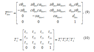
where cθ and sθ refers to cosθ and sinθ respectively.

Dynamic parameter estimation

The Linear-least-square (LLS) method together with an optimized excitation trajectory was used for dynamic parameter estimation of the robot manipulator. LLS requires that the model equations are linear with respect to dynamic parameters and it is sensitive to noise in the measured data. [34] observed that the actuator forces of an industrial manipulator are linear functions of dynamic parameters, [4] inferred that reformulating the Newton-Euler dynamic model such that the link inertia tensors are expressed about the link coordinate frames instead of the center of the links’ mass, would result in a linearized Newton-Euler formulation. Equations (11-14) presents a summarized Newton-Euler formulation in the form of observation matrix. For detailed information on linearizing the Newton-Euler equation, see [4] and [34].

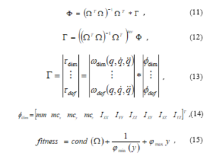
where Γ is the compound torque for the manipulator comprising of individual joint torques τ, the compound observation matrix Ω comprises of individual joint vectors ω(q, q̇, q̈), and is a function of the joint position, velocity, and acceleration only. ϕ is a vector of unknown robot parameters for each link that require to be identified, it includes link mass mm, first moments [mc_x mc_y mc_z]^T along the x-y-z axis, and six inertia tensor I_ij, these compose the compound vector of unknown parameters Փ. The intelligent swarm-based algorithm would be required to minimize the condition number of the observation matrix while maximizing the smallest singular value and minimizing the largest singular value. Therefore, the fitness function would be as described in (15).

Exciting trajectory

A modified Fourier series (MFS) formulation was used to define the excitation trajectory with a cubic polynomial. The equation of motion for the trajectory of the first three joints are given in (16-18), a circular trajectory path was implemented so as to allow continuous trajectory tracking of the robot during experimentation. The trajectory is to be optimized by applying the eMuPSO algorithm to minimizing the condition number of the observation matrix. The trajectory is implemented in Cartesian space, and joint positions are determined from inverse kinematic solutions. The wrist of the manipulator has a z-x-z orientation, therefore the excitation trajectory along the x and y axis can be derived independently from (16) and (17) while that of the z axis is estimated from (19), where d6 is the offset length of the sixth link of manipulator (see DH parameters) and t₁₄ is the position coordinate of transformation matrix T₄⁰ from the Base to Link-04.

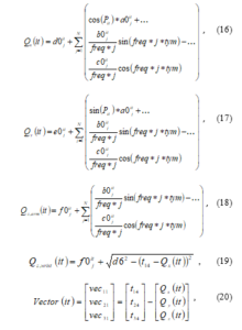
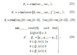
where Q describes the trajectory in Cartesian space such that [Q_x, Q_y, Q_z]^T are the x-y-z coordinates of Q, P is the polynomial, the variables a0 is the radius, b0 and c0 are the coefficients of the MFS while the variables d0, e0, and f0 are the x-y-z position coordinates of the excited trajectory.  j = 1,2…N denotes the harmonics of the MFS, while the index of time segment/period is denoted as it; freq is the fundamental frequency and tym is the period. The joints 4, 5, and 6 coincident at the joint 5, described by the transformation matrix T₄⁰ in (10). The inverse kinematic solution of these joints can be estimated given the orientation matrix, but in this case only the position vector is known (i.e. [Qx, Qy, Qz]^T). Therefore, the rotation angles of the joints at the wrist would be estimated from (20-23), and the orientation matrix is evaluated by substituting θ in (9) then inverse kinematics can be subsequently evaluated. To achieve continuity along the tool-path, the initial and final conditions of the trajectory must be the same as described in the conditions in (24). The initial and final values for the circular trajectory P are set as 0 and 2π radians, 3 harmonics for the coefficients of MFS were used (N=3), and the fundamental frequency is 0.6283 with a period of 10 seconds.

4. Results

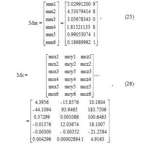
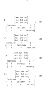
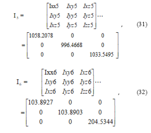
The eMuPSO algorithm was first implemented together with the LLS for optimizing the observation matrix and dynamic parameter estimation of all the six links of the 6DOF robot manipulator. The ideal parameters of the manipulator are given in (25-32). Then the proposed algorithm was finally implemented in evaluating thirty-six benchmark functions including twenty-four variable-dimension benchmark functions and twelve constant-dimension benchmark functions. The variable dimension benchmark functions consist twelve functions each, of unimodal and multi-modal roles (a full description of all benchmark function used are given in the appendix).

The results were compared with the Standard PSO (PSO) [35] and four other swarm-based EAs including the Whale Optimization Algorithm (WOA) [36], Grey Wolf Optimization (GWO) [37], Grass-hopper Optimization Algorithm (GOA) [38], and the Differential Evolution (DE) algorithms [39].

4.1. Dynamic Parameter Estimation

Generating initial elite particles

Parameter estimation was in two stages; initial elite particles were first generated which were then used to generate the swarm for parameter estimation. This reduces the probability for the algorithm to run into stagnation. A swarm of ten particles was first generated for each variable (a0, b0, …, f0). From inverse kinematics, the joint conditions (position, velocity and acceleration) corresponding to the generated trajectory of each set of particle is estimated and compared with the stated constraints in (24).  Trajectories that do not meet the constraints are flagged and a penalty was introduced.

The fitness function for this swarm is a measure of the degree of compliance of the generated trajectory with the stated robot constraints. If a trajectory is found to completely satisfy these constraints, the variables corresponding to such trajectory is elevated to elite status and a new particle is generated to replaces that particle, else, the entire swarm’s velocity and position is updated in accordance with PSO. Elite particles should be generated within 5-10 iteration if the minimum and maximum limits of the variables are carefully selected. This algorithm is terminated when 5 elite particles have been generated. The variable limits are set at ±10. While the variables a and b span between negative and positive limits, others must always be positive.

Optimizing the excitation trajectory

A swarm of 20 particles is generated from the previously generated initial elite particles through Gaussian mutation. Similar to previous procedures, the boundary conditions are set, joint conditions corresponding to each generated trajectory is estimated, again penalties are introduced to make trajectories that do not satisfy the constraints in (24) less likely to be selected as exemplars. The fitness function for this swarm is evaluated according to (15). The swarm of the algorithm is mutated at 10 iterations after stagnation (i.e. G=10).

Parameter estimation

The dynamic parameters of a 6DOF manipulator was estimated in two stages, the last three links corresponding to the wrist were first estimated followed by the first three links corresponding to the arm of the manipulator. A numeric technique for reducing the observation matrix to a minimum linear combination of identifiable parameters was implemented as described in [40] where three empty matrices were created corresponding to identifiable parameters, unidentifiable parameters, and identifiable parameters in linear combinations. Understanding that the rank of the observation matrix is equal to the number of identifiable parameters, the norm of each column of the observation matrix is determined independently. The columns with zero norms represent coefficients of unidentifiable parameters and are moved to the matrix of unidentifiable parameters, else it is added to the matrix of identifiable parameters. Note that the initial rank of the empty matrix of identifiable parameters is zero, if the newly added column does not increase the rank of the matrix of identifiable parameters, it is moved to the matrix of identifiable parameters in linear combination. The eMuPSO was used to select the trajectory that best optimizes the observation matrix. Removing unidentifiable parameters from the observation matrix increases estimation accuracy. In the first estimation stage (wrist), out of the 30 unknown parameters at the wrist, 15 were independently identifiable, 7 were identifiable in linear combination, while 8 were unidentifiable. Out of the 7 parameters that were identifiable in linear combination, it was observed that for most elite particles, 5 were identifiable with lower errors. The 15 independently identifiable parameters include Iyy4, Ixz4, mx5, Ixx5, Iyy5, Izz5, Ixy5, Ixz5, Iyz5, mcx6, mcy6, Iyy6, Izz6, Ixz6, and Iyz6. The 7 parameters identifiable in linear combination include mcy4, mcy5, mcz5, mm6, mcz6, Ixx6, and Iyz6. It was found that Ixx6 and Iyz6 were identified with very large errors for most elite particles. In the second estimation stage (arm), 20 parameters were independently identifiable, 2 were identifiable in linear combinations while 8 were unidentifiable. All parameters were identified with little errors. The 22 identified parameters include mcy1, Iyy1, mm2, mcx2, mcy2, mcz2, Iyy2, Izz2, Ixz2, Iyz2, mm3, mcx3, mcy3, mcz3, Ixx3, Iyy3, Izz3, Ixy3, Ixz3, Iyz3, Ixz1, and Ixx2.

Figure 2.0 (a) and (b) show the convergence plot at the wrist and at the arm of the manipulator respectively. The eMuPSO was populated with twenty particles in thirty iterations and five runs. The Figure 2.0 shows all five runs, the sixth being the average of all five runs. It would be observed that in the third run of Figure 2.0 (a), the algorithm converges to the global minimum solution in eight iterations, then it is mutated in the 14^th iteration where it stagnates until it is mutated again in the 24^th iteration. The best solutions are stored in the archive before mutation. The Figure 2.0 (b) show less agitation of the algorithm signifying less mutation and simpler analysis.

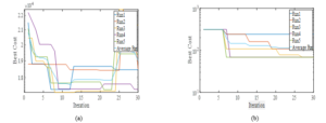
Figure 2: Convergence plot of the observation matrices (a) at the wrist, and (b) at the arm.

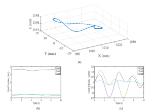
Figure 3: Excitation trajectory for the links at the wrist of manipulator. (a) Trajectory in Cartesian space (b) Joint displacement (c) Joint velocities

Table 2: Dynamic parameter estimation for the last three joints of a 6 DOF industrial robot

Parameter	Elite Particles (wrist)
	1	2	3	4	5	6
a0(1)	-3.8711	-8.7566	-6.1829	-4.824	-6.7566	-4.4276
a0(2)	9.8782	1.1156	5.7223	-2.4838	3.1156	4.0066
a0(3)	0.42207	4.5867	-4.0733	-3.0035	3.748	-5.7368
b0(1)	2.1907	2.8328	4.9482	2.6421	4.7319	6.1336
b0(2)	-3.5264	-7.3354	-2.4158	-1.0079	-5.3354	5.1722
b0(3)	-2.293	-7.4121	0.31497	-3.5628	-5.4121	0.91808
c0	6.5802	5.4755	6.423	6.8105	5.0595	2.9898
d0	6.5802	3.1097	6.423	0.85837	5.0595	2.9898
e0	0	0	0	0	0	0
f0	t34	t34	t34	t34	t34	t34
fitness	418.354	401.380	357.993	351.894	349.889	297.128
condition number	154.591	152.878	156.902	157.041	155.063	154.087
Error(20)	10.8120	188.679	14.5859	99.1558	86.8486	25.3959
Error(22)	2220.44	16789.5	529.495	4568.45	8777.48	44.3582

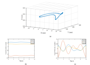
Figure 4: Excitation trajectory for the links at the arm of manipulator. (a) Trajectory in Cartesian space (b) Joint displacement (c) Joint velocities

Table 3: Dynamic parameter estimation for the first three joints of a 6 DOF industrial robot

Parameter	Elite Particles (Arm)
	1	2	3	4	5	6
a0(1)	-1.2742	5.2376	-3.2742	-2.8265	0.72577	-3.2742
a0(2)	-6.5754	6.2129	-4.5754	-6.5754	-8.5754	-8.5754
a0(3)	-9.0638	8.2042	-7.0638	-9.0638	-6.8925	-6.7108
b0(1)	-0.4967	6.2173	1.5033	-0.4967	1.5033	-2.4967
b0(2)	4.5411	-2.6712	2.6293	2.9774	2.5411	6.5411
b0(3)	-1.6233	-7.73	-0.74646	1.2535	-3.6233	0.37674
c0	3.0295	1.4518	1.0295	1.7199	1.0295	1.0295
d0	0	0	0	0	0	0
e0	173.11	101.03	184.34	187.21	188.04	166.14
f0	5.7001	6.0889	1.0295	1.7199	1.0295	1.0295
fitness	293.392	199.588	145.3132	103.235	70.9066	64.7651
condition number	53.5757	44.7731	26.41273	17.8764	13.4862	11.8133
Error(20)	0.00270	0.00286	0.035218	0.01955	0.03211	0.00822
Error(22)	0.00460	0.00766	0.074774	0.03507	0.08359	0.01544

Tables 2 and 3 presents the parameters of the non-dominated elite solutions for the joints at the arm and wrist of the manipulator, including the three harmonics each for a0 and b0, with corresponding fitness values, condition number of the observation matrix and cumulative errors for the best 20 identified parameters and for all 22 identified parameters. Figure 3.0 (a) presents the resultant trajectory in Cartesian space for the 5^th elite particle at the robot’s wrist, showing a somewhat circular continuous trajectory with fluctuations that are typical of FFS. Figures 3.0 (b) and (c) show the position and velocity of the three joints at the robot’s wrist in joint space, while Figure 4.0 shows the equivalent for the 1^st elite particle at the robot’s arm. From the results presented in Table 2 (at the wrist), it would be observed that while the 6^th elite particle has the lowest fitness value and the lowest cumulative estimation error for all the 22 identified parameters, the 2^nd elite particle presents the trajectory with the lowest condition number, and the 1^st elite particle presents the lowest cumulative estimation error for the 20 best identified parameters. Likewise, in Table 3 (at the arm), although all the 22 identifiable parameters were identified with higher accuracy, yet it would also be observed that the 6^th elite particle has the lowest fitness and presents the trajectory with the lowest condition number, but the 1^st elite particle presents the lowest cumulative estimation errors for both the 20 best identified parameter and the 22 identifiable parameters. This supports the observation of [41] that the best solution does not guarantee the global minimum solution because the dynamic optimization problem is not convex.

4.2. Benchmark Function Analysis

A total of thirty-six benchmark functions (BF) were evaluated, and the results presented in Tables 4-6. Reference [2] showed that accuracy and convergence time are paramount in robot analysis, the average and standard deviations alone do not completely describe the results, and some solutions with good averages are incapable of finding the global minimum solution (inaccurate). Therefore, the minimum values are also presented in the tables. The solution that best minimizes the function is presented in bolded font. From the Table 4, in the unimodal BF analysis, all the algorithms satisfactorily found the minimized solution for the function f6; eMuPSO, PSO, and DE equally minimized the function f7 while GWO and WOA equally minimized the function f11. WOA and GWO had the best performance, producing the best minimizing solutions for five out of twelve unimodal BF each. WOA dominated other algorithms in f1, f3, and f12 functions, tied with GWO in f11 and tied with all other metaheuristics in f6. While GWO dominated other metaheuristics in f8, f9, and f10. Therefore, WOA and GWO dominated other algorithms in three unimodal BF, tied in two BF and were dominated in seven BF each as elaborated in Table 7. The PSO dominated other metaheuristics in f4 and f5, while eMuPSO was dominant in f2. Both tied with other metaheuristics in f6 and f7 and were dominated in eight and nine unimodal BF respectively. From the Table 5, in the multimodal BF analysis, it can be observed that the eMuPSO and PSO tied in f1, f4, and f12; PSO, WOA, and GWO tied in f2; WOA and GWO tied in f3; eMuPSO, PSO and GOA tied in f5; all the metaheuristics except GWO and DE tied in f6, eMuPSO and DE tied in f9, and all the metaheuristics except GOA tied in f11. eMuPSO had the best performance producing the best minimum results on eight out of twelve multimodal BF, followed by PSO, WOA, and GWO producing the best minimum solutions for seven, five, and four multimodal BF respectively. eMuPSO dominated other metaheuristics on f10 and tied with other metaheuristics on seven multimodal BF. PSO did not dominate other metaheuristics on any of the multimodal BF, but tied on seven and was dominated in five BF, WOA was dominant on f7, tied with other metaheuristics on 4 Multimodal BF and was dominated in 7 BF. GWO was dominant on f8, tied with other metaheuristics on 3 BF, and was dominated on 8 BF. From the Table 6, in the constant dimension BF analysis, eMuPSO and PSO tied in producing the best minimizing solution for f1 and f6, all metaheuristics except GOA and GWO tied on f2; eMuPSO, PSO and DE tied on f3, f5, f7, f8, f9, f11. All the metaheuristics except WOA and GWO tied on f4 and f12. eMuPSO once again had the best performance producing the best minimum solutions for all twelve BF, dominated other metaheuristics in f10, and tied in eleven BF, followed by PSO and DE producing the best-minimized solution for eleven and nine BF respectively. Compared to other algorithms, WOA and GWO performed well in the unimodal BF analysis but performed poorly in the constant-dimension BF analysis. After numerous experiments, at various dimension sizes, it can be suggested that the WOA algorithm is convenient for analyzing optimization problems with high dimensionality (especially unimodal roles), but may not necessarily maintain its lead when the dimensionality is low, while the proposed eMuPSO is convenient for analyzing optimization problems with lower dimensionality. Compared to other EAs, the eMuPSO and PSO algorithms performed averagely in the unimodal BF evaluations but were excellent in analyzing multimodal and constant-dimension BF. DE performed poorly in the unimodal and multimodal BF, performed well in the constant-dimension BF analysis.

The Wilcoxon signed-rank test was performed at a 5% significance level to compare the results of each run and decide on the significance of the results, and the p-values are reported in Table 8. In the statistical analysis, the best algorithm in each test function is the algorithm with the best average value, the best algorithm is compared with other algorithms independently. For instance, if eMuPSO is the best algorithm, pairwise comparison is done between eMuPSO/PSO, eMuPSO/GOA, and so on. Observe that since the best algorithm cannot be compared with itself, N/A with bold font size has been assigned to it. From Table 8, in the unimodal statistical analysis (F1-F12) WOA algorithm was most significant in six out of twelve BF as elaborate in Table 9. SPSO and GWO were significant in four functions each, while DE and eMuPSO were significant in three and two of the functions respectively. In the multimodal statistical analysis (F13-F24), the eMuPSO and DE were most significant in six out of the twelve BF each, followed by WOA with five BF, while SPSO and GWO were most significant in 3 of the BF each. In the constant-dimension statistical analysis (F25-F36), the eMuPSO and DE remained most significant for ten out of the twelve BF each, followed by the SPSO with 8 BF, GOA was most significant in 2 of the BF, while others were significant in only one each of the benchmarks functions.

Table 4: Unimodal benchmark function analysis.

Unimodal Benchmark Functions		Evolutionary Algorithms
		eMuPSO	PSO	WOA	GWO	GOA	DE
F1: Sphere	Min	2.00E-12	4.90E-44	0	2.85E-240	2.25E-06	0.001903
	Ave	9.46E-08	5.44E-42	0	1.91E-232	8.66E-05	0.031038
	StDev	3.13E-07	2.23E-41	0	0	9.17E-05	0.039287
F2: Beale	Min	1.67E-08	7.70E-08	0.000176	6.42E-05	0.000149	3.147E-08
	Ave	0.0178315	0.015488	0.026001	0.005977	0.035998	1.43E-07
	StDev	0.0308013	0.029336	0.044659	0.0154745	0.038128	2.13E-07
F3: Matyas	Min	1.69E-12	2.12E-24	0	1.33E-143	1.42E-06	3.50E-07
	Ave	3.42E-09	1.07E-18	0	1.57E-120	1.55E-05	6.23E-06
	StDev	7.91E-09	5.33E-18	0	4.10E-120	1.51E-05	5.08E-06
F4: Rosenbrook	Min	10.167783	0.087952	14.80708	15.116454	13.29022	6.665086
	Ave	28.023866	6.257364	15.61825	16.217369	258.643	28.08251
	StDev	32.409539	3.514322	0.417166	0.6497502	480.0779	31.98284
F5: Step 2	Min	3.91E-10	0	1.38E-05	1.91E-07	7.31E-07	0.004025
	Ave	8.03E-08	0	4.99E-05	0.1749605	0.000109	0.047807
	StDev	1.77E-07	0	3.02E-05	0.1875981	0.000145	0.055443
F6: Scahffer 2	Min	0	0	0	0	0	0
	Ave	0	0	0	0	0	0
	StDev	0	0	0	0	0	0
F7: Scahffer 3	Min	-3.37E-4	-3.37E-4	-3.37E-4	-3.37E-4	-3.37E-4	-3.37E-4
	Ave	-3.37E-4	-3.37E-4	-3.36E-4	-3.37E-4	-3.37E-4	-3.37E-4
	StDev	1.65E-19	1.65E-19	3.00E-06	3.45E-08	1.08E-09	1.65E-19
F8: Scwefel 1.2	Min	0.0003765	1.92E-11	0.317571	7.14E-99	1.759081	0.003903
	Ave	0.0071479	4.45E-09	207.2391	4.23E-82	33.02237	0.079942
	StDev	0.0069211	6.37E-09	408.9857	2.15E-81	28.64997	0.090924
F9: Scwefel 2.21	Min	0.370036	9.76E-10	1.62E-09	8.56E-66	0.018632	0.179791
	Ave	1.0249904	1.39E-08	4.32931	1.20E-62	1.084041	2.315132
	StDev	0.5007591	1.17E-08	9.450776	4.98E-62	1.537078	2.441406
F10: Scwefel 2.22	Min	0.0027291	5.00E-26	2.0800E-322	4.67E-136	0.018623	0.077971
	Ave	0.0326953	2.66E-24	2.7900E-321	1.61E-133	0.192329	1.517522
	StDev	0.0266489	5.88E-24	0	5.42E-133	0.578804	2.606056
F11: De Jong 4	Min	2.35E-22	1.53E-79	0	0	1.40E-13	5.83E-10
	Ave	3.14E-14	4.80E-73	0	0	2.75E-09	0.117002
	StDev	9.95E-14	1.73E-72	0	0	3.50E-09	0.640849
F12: Axis Parallel	Min	4.79E-12	2.48E-46	0	2.61E-241	3.93E-05	6.28E-05
	Ave	2.12E-08	2.71E-43	0	2.61E-235	0.001067	0.000993
	StDev	6.13E-08	9.27E-43	0	0	0.001414	0.001253

Table 5: Multimodal benchmark function analysis.

Multimodal Benchmark Functions		Evolutionary Algorithms
		eMuPSO	PSO	WOA	GWO	GOA	DE
F13: Easom	Min	0	0	3.26E-15	7.77E-12	2.11E-16	NaN
	Ave	0	0	0.023333	1.00E-09	0.086667	NaN
	StDev	0	0	0.043018	9.16E-10	0.034575	NaN
F14: Griewank	Min	2.00E-07	0	0	0	0.000577	0.011976
	Ave	0.0343134	0.015987	0.001742	0.0001222	0.04842	0.147971
	StDev	0.0330935	0.017756	0.009541	0.0006694	0.06238	0.143891
F15: Rastrigin	Min	8.9546265	7.959672	0	0	31.83894	9.732789
	Ave	17.378784	16.01883	0	0	67.56469	36.96119
	StDev	5.8526738	5.267084	0	0	29.12814	22.58322
F16: Pen Holder	Min	-9.04E-08	-9.04E-08	2.87E-07	0.0393752	0.026031	NaN
	Ave	0.0168779	0.001703	0.029721	0.0652148	0.082208	NaN
	StDev	0.0251307	0.004706	0.02437	0.0179396	0.034506	NaN
F17: Test-tube Holder	Min	-2.04E-08	-2.04E-08	-2.04E-08	-2.04E-08	-2.04E-08	-2.040E-08
	Ave	-2.04E-08	-2.04E-08	0.000198	-1.63E-08	0.002207	-1.50E-05
	StDev	0	0	0.000604	4.80E-09	0.00908	3.01E-05
F18: Egg Holder	Min	0	0	0	1.03E-10	0	NaN
	Ave	69.652218	52.92821	1.14E-13	25.398919	149.1868	NaN
	StDev	77.530967	74.41267	1.16E-13	50.110379	130.2925	NaN
F19: Damavandi	Min	2	2	0.009163	2.0000051	2	2.000002
	Ave	2	2	0.278923	2.2578664	2.000002	2.000018
	StDev	3.27E-10	0	1.197583	1.412306	3.83E-06	1.32E-05
F20: Cross-Leg Table	Min	0.0037107	0.049876	0.099255	0	0.09978	0.0150
	Ave	0.0603736	0.084285	0.099835	0.0832343	0.099862	0.011415
	StDev	0.0271336	0.019337	0.000111	0.0378599	2.45E-05	0.006958
F21: Bucking 4	Min	0	1.47E-90	2.20E-11	1.58E-08	3.80E-08	0
	Ave	0	5.03E-79	1.17E-06	1.15E-06	0.00028	0
	StDev	0	2.35E-78	1.28E-06	1.26E-06	0.000495	0
F22: Bucking 6	Min	0.0023858	0.003192	0.003289	0.092071	0.0065	0.013404
	Ave	0.1010663	0.119555	0.124073	0.152622	0.098243	0.097272
	StDev	0.0585834	0.074511	0.08727	0.0926189	0.066986	0.055002
F23: Cosine	Min	0	0	0	0	1.94E-15	0
	Ave	0.0084647	0	0	0	0.08306	0
	StDev	0.0080534	0	0	0	0.05875	0
F24: Modified Rosenbrook	Min	3.4040243	3.404024	3.404024	3.4040243	3.404024	3.404024
	Ave	4.8692154	5.80161	3.404024	6.8672033	7.000974	3.404024
	StDev	1.9585576	1.991086	4.00E-08	1.3815921	1.219484	1.88E-15

Table 6: Constant-dimension benchmark function analysis.

Constant-Dimension Benchmark Functions		Evolutionary Algorithms
		eMuPSO	SPSO	WOA	GWO	GOA	DE
F25: Paviani	Min	-2.34E-06	-2.34E-06	4.52E-06	1.91E-05	-2.34E-06	NaN
	Ave	-2.34E-06	-2.34E-06	0.000137	4.28E-05	-2.34E-06	NaN
	StDev	5.70E-15	3.54E-15	0.00013	2.09E-05	2.03E-11	NaN
F26: Modified Ackley	Min	0	0	0	1.53E-10	1.78E-15	0
	Ave	0	0	2.01E-10	4.45E-09	3.00E-14	0
	StDev	0	0	3.77E-10	3.79E-09	2.01E-14	0
F27: Camel 6 Hump	Min	2.22E-16	2.22E-16	1.11E-15	1.11E-13	4.44E-16	2.22E-16
	Ave	2.22E-16	2.22E-16	5.03E-13	3.93E-10	8.44E-16	2.22E-16
	StDev	0	0	1.25E-12	4.48E-10	3.37E-16	0
F28: Branin Rcos	Min	-2.26E-11	-2.26E-11	-2.26E-11	1.84E-10	-2.26E-11	-2.26E-11
	Ave	-2.26E-11	-2.26E-11	6.93E-09	1.94E-08	-2.26E-11	-2.26E-11
	StDev	0	0	1.32E-08	2.29E-08	4.85E-15	0
F29: Hartmann 3	Min	-1.78E-05	-1.78E-05	-1.78E-05	-1.78E-05	-1.78E-05	-1.78E-05
	Ave	-1.78E-05	-1.78E-05	0.000528	0.0005009	0.051517	-1.78E-05
	StDev	0	0	0.001523	0.0017303	0.196121	0
F30: Hartmann 6	Min	0	0	9.46E-07	4.68E-08	6.22E-15	4.44E-16
	Ave	0.0435941	0.047557	0.041273	0.056637	0.043647	0.11493
	StDev	0.0582734	0.059241	0.059382	0.0745266	0.058344	0.021707
F31: Shekel 5	Min	0	0	2.36E-06	2.51E-06	6.04E-14	0
	Ave	1.5943441	2.514812	0.81061	0.6767119	4.505148	0
	StDev	2.7615053	3.018129	2.487387	1.7547512	3.369024	0
F32: Shekel 7	Min	-20.80588	-20.80588	-20.80588	-20.80588	-20.80588	-20.80588
	Ave	-19.2602	-19.6892	-20.62807	-20.80587	-17.28696	-20.80588
	StDev	2.9070217	2.583984	0.970316	1.00E-05	3.854556	3.61E-15
F33: Shekel 10	Min	-2.20E-07	-2.20E-07	2.50E-06	1.27E-06	-2.20E-07	-2.20E-07
	Ave	0.4489944	1.336099	0.455673	1.37E-05	4.623238	-2.20E-07
	StDev	1.7463952	2.782463	1.750715	6.81E-06	3.885799	5.42E-16
F34: Perm	Min	1.00E-30	1.81E-26	0.067631	0.0001552	0.00023	0.0049
	Ave	0.042594	0.03135	2.678428	1.3509178	0.046792	0.006286
	StDev	0.095434	0.089466	3.288481	2.9794594	0.093625	0.007091
F35: Goldstein Price	Min	-8.08E-14	-8.08E-14	5.46E-11	5.70E-10	-7.02E-14	-8.08E-14
	Ave	-7.87E-14	-7.86E-14	5.70E-07	1.04E-06	2.7	-7.93E-14
	StDev	9.85E-16	8.92E-16	1.13E-06	9.80E-07	14.78851	8.83E-16
F36: Langerman 5	Min	0.3033287	0.303329	0.694475	0.3033287	0.303329	0.303329
	Ave	0.5761576	0.61325	1.021407	0.5757514	0.742518	0.329675
	StDev	0.3298947	0.33584	0.186392	0.3026761	0.321734	0.10027

Table 7: Summary of benchmark function evaluations.

Summary of Benchmark Function Analysis		Evolutionary Algorithms
		eMuPSO	PSO	WOA	GWO	GOA	DE
Minimum function Evaluations	Unimodal	1/2/9	2/2/8	3/2/7	3/2/7	0/1/11	0/2/10
	Multimodal	1/7/4	0/7/5	1/4/7	1/3/8	0/3/10	0/3/9
	Constant Dim.	1/11/0	0/11/1	0/1/11	0/0/12	0/2/10	0/9/3
	Total	3/20/13	2/20/14	4/7/25	4/5/27	0/6/30	0/14/22

Table 8: p-Values obtained from Wilcoxon signed rank pairwise test.

Wilcoxon signed rank pairwise test (Benchmark Functions)	Evolutionary Algorithms (P_val)
	eMuPSO	SPSO	WOA	GWO	GOA	DE
F1: Sphere	1.73E-06	1.73E-06	NA	1.73E-06	1.73E-06	1.73E-06
F2: Beale	NA	1.73E-06	1.73E-06	1.73E-06	1.73E-06	1
F3: Matyas	1.73E-06	1.73E-06	NA	1.73E-06	1.73E-06	1.73E-06
F4: Rosenbrook	1.92E-06	NA	1.73E-06	1.73E-06	1.73E-06	1.92E-06
F5: Step 2	1.73E-06	NA	1.73E-06	1.73E-06	1.73E-06	1.73E-06
F6: Scahffer 2	NA	1	1	1	1	1
F7: Scahffer 3	NA	1	1.73E-06	1.73E-06	1.73E-06	1
F8: Scwefel 1.2	1.73E-06	1.73E-06	1.73E-06	NA	1.73E-06	1.73E-06
F9: Scwefel 2.21	1.73E-06	1.73E-06	1.73E-06	NA	1.73E-06	1.73E-06
F10: Scwefel 2.22	1.73E-06	1.73E-06	NA	1.73E-06	1.73E-06	1.73E-06
F11: De Jong 4	1.73E-06	1.73E-06	NA	1	1.73E-06	1.73E-06
F12: Axis Parallel	1.73E-06	1.73E-06	NA	1.73E-06	1.73E-06	1.73E-06
F13: Easom	NA	1	1.67E-06	1.73E-06	1.98E-07	NaN
F14: Grievant	1.73E-06	5.94E-05	1	1	1.73E-06	1.73E-06
F15: Rastrigin	1.73E-06	1.73E-06	NA	1	1.73E-06	1.73E-06
F16: Pen Holder	NA	1.01E-06	1.73E-06	1.73E-06	1.73E-06	NaN
F17: Test-tube Holder	0.015625	0.015625	1.73E-06	1.73E-06	5.06E-06	1
F18: Egg Holder	NA	0.000375	0.014795	0.002585	4.73E-06	NaN
F19: Damavandi	3.11E-05	3.11E-05	NA	2.84E-05	3.11E-05	3.11E-05
F20: Cross-Leg Table	1.92E-06	1.73E-06	1.73E-06	7.69E-06	1.73E-06	1
F21: Bucking 4	1.73E-06	1.73E-06	1.73E-06	1.73E-06	1.73E-06	1
F22: Bucking 6	NA	0.19861	0.14704	0.010444	0.53044	0.734325
F23: Cosine	NA	1	1	1	1.73E-06	1
F24: Modify Rosenbrook	NA	3.38E-05	1.73E-06	1.73E-06	1.72E-06	1
F25: Paviani	1.73E-06	1	1.73E-06	1.73E-06	1.73E-06	NaN
F26: Modified Ackley	NA	1	2.56E-06	1.73E-06	1.73E-06	1
F27: Camel 6 Hump	NA	1	1.73E-06	1.73E-06	1.50E-06	1
F28: Branin Rcos	NA	1	1.73E-06	1.73E-06	0.007813	1
F29: Hartmann 3	NA	1	1.73E-06	1.73E-06	1.73E-06	1
F30: Hartmann 6	0.877403	0.106394	1	0.544006	0.082206	0.000616
F31: Shekel 5	0.25	0.000244	1.73E-06	1.73E-06	1.73E-06	1
F32: Shekel 7	NA	0.0625	1.73E-06	1.73E-06	1.71E-06	1
F33: Shekel 10	0.375	0.007813	1.73E-06	1.73E-06	1.73E-06	1
F34: Perm	0.24519	0.236936	1.73E-06	0.000388	0.093676	1
F35: Goldstein Price	0.000509	0.004651	1.73E-06	1.73E-06	1.73E-06	1
F36: Langerman 5	0.165027	0.025637	1.73E-06	0.001382	0.000148	1

Table 9: Summary of Wilcoxon signed rank pairwise test evaluations.

Summary of Wilcoxon signed rank pairwise test		Evolutionary Algorithms
		eMuPSO	PSO	WOA	GWO	GOA	DE
Wilcoxon Signed Rank test	Unimodal	0/2/10	2/2/8	4/2/6	2/2/8	0/1/11	1/2/9
	Multimodal	2/4/6	0/3/9	1/4/7	0/3/9	0/1/11	2/4/6
	Constant Dim.	0/10/2	1/7/4	0/1/11	0/1/11	0/2/10	1/9/2
	Total	2/16/18	3/12/21	5/7/24	2/6/28	0/4/32	4/15/17

4.3. Convergence Analysis

In Figure 5, the unimodal convergence plot analysis, it can be observed that eMuPSO was dominant in f2, tied with other metaheuristics in f6 and f7, produced the second-best minimum solution for f4 and f5, and the third-best minimum solution for f8. A large overshoot can also be observed in the results of f7. In Figure 6, the multimodal convergence plots, eMuPSO dominated others in f10 and tied in f1, f4, f5, f6, f9, f10, f11. eMuPSO produced the second-best minimized solution in f8. All the algorithms except WOA stagnated at the local minimum in f7. In Figure 7, the Constant-dimension benchmark function convergence plots, eMuPSO best minimized all twelve BMF dominating others in f10. Overshoot can be observed in the results of eMuPSO in f25, f28, f29, f33, and f35. Similarly, an overshoot can also be observed in the results of WOA in f28 and f29. In the convergence plots presented, it can be seen that the GOA and GWO produced the slowest converging results, this is most evident in f13, f16, f18, f22, and most of the constant-dimension benchmark functions. This suggests good exploration capabilities of the swarms. Whereas eMuPSO, PSO, and DE produced the fastest converging results. In robot analysis speed and accuracy are required, therefore the best algorithm has to make a balance between fast convergence speed and good exploration tendencies.

5. Conclusion

An enhanced PSO algorithm was proposed with a Gaussian mutation and an archive elite learning (eMuPSO), the parameters and dynamic update technique were optimized for robot analysis. The parameter identification problem of robot manipulators is generally computationally demanding, therefore finding a computationally efficient solution is important for which swarm-based algorithms are suitable. In Dynamic parameter estimation, excitation trajectory was optimized using the proposed eMuPSO, it allowed the swarm to be populated with fewer particles thereby requiring less computational time. The mutation function allowed a wholesome search of the solution space. The LLS method was subsequently used to estimate the dynamic parameters of a 6DOF industrial robot manipulator where it was seen that estimation errors are larger at the wrist of the manipulator. Parameter estimation accuracy is better at the arm with less dexterity, while the total estimation accuracy for the 6DOF manipulator is deteriorated by the cumulative estimation errors at the wrist with increased dexterity. This suggests that larger DOF manipulators would be suitable for manufacturing, agriculture and other industrial applications, but may not be suitable for high end application that are keen on accuracy like medical operations, airplane manufacture, etc. The eMuPSO particularly gives a scientist the advantage of choosing from the set of elite particles, the solution that best solves the desired problem. The eMuPSO is therefore capable of analyzing both kinematic and dynamic robot problems of robot manipulators. Further experimentation showed that the landscape of the solution space for robot optimization problems are non-linear, non-separable and multi-modal with multiple possibilities of sub-optimal solutions (local minimizers) some of which are very steep. When a solution approaches the vicinity of these steep local minimizers, it easily falls into its trap and it is usually very difficult to break out of such stagnation without artificial perturbation, resulting to the failure of most evolutionary algorithms in analyzing robot optimization problems. The performance of the eMuPSO can be related to its origins. The parameters of the eMuPSO was derived experimentally by comparing the performance of various robot manipulator configurations as described in [2]. The robot optimization problem is a non-linear and multi-modal problem with dimension size usually less than twenty. Robot manipulator problems are generally computational demanding, therefore a fast convergence time and high accuracy are important. The eMuPSO best showed its veracity in analyzing multimodal and constant dimension BF. PSO and DE performed well in constant dimension BF. It would also be observed that the proposed eMuPSO cannot drill a solution below 1E-30, this is also suitable for robot analysis because the solution to robot optimization problems is usually in the range of 1E-10.

For a successful dynamic parameter estimation analysis, the following should be carefully observed.

• It is recommended to keep either d0 or e0 equal to zero to avoid singularity so that the excitation trajectory is limited two quadrants on the x-y plane.
• It would be keen to differentiate between dynamic and kinematic DH-parameters. When determining the position coordinated of the robot manipulator, the sum of lengths of the 3^rd and 4^th links make up d4, while during dynamic analysis this results in actuator torque errors. Likewise, the length d6.

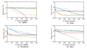
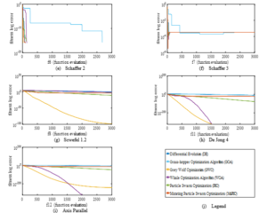
Figure 5: Convergence analysis for unimodal benchmark functions.

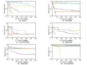
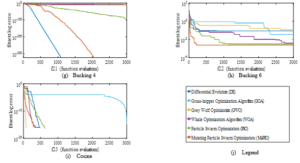
Figure 6: Convergence analysis for multimodal benchmark functions.

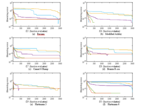
Figure 7: Convergence analysis for constant-dimension benchmark functions.

• When determining the 6^th joint angle from the excitation trajectory vector with (27), the initial joint position is unknown, so it is recommended to assume the initial joint position at the first segment (@ it = 1) is equal to the joint position at the last time segment to reduce the overshoot in velocity.

Funding

This research was funded by the National Natural Science Foundation of China, grant number 51875166.

Conflict of Interest

The authors declare no conflict of interest.

Acknowledgment

I would like to first acknowledge my late mum whose unflinching support kept me going against all odds and who unfortunately is no more with us to witness my achievements, my lovely wife and children who were patient with me through these trying times and finally to Prof. Shi for giving me the opportunity and finding me worthy.

1. A. Umar, Z. Shi, W. Wang, Z.I.B. Farouk, “A Novel Mutating PSO Based Solution for Inverse Kinematic Analysis of Multi Degree-Of-Freedom Robot Manipulators,” Proceedings of 2019 IEEE International Conference on Artificial Intelligence and Computer Applications, ICAICA 2019, 459–463, 2019, doi:10.1109/ICAICA.2019.8873449.
2. A. Umar, Z. Shi, A. Khlil, Z.I.B. Farouk, “Developing a New Robust Swarm-Based Algorithm for Robot Analysis,” Mathematics, 8(2), 158, 2020, doi:10.3390/math8020158.
3. B. Armstrong, “On Finding Exciting Trajectories for Identification Experiments Involving Systems with Nonlinear Dynamics,” The International Journal of Robotics Research, 8(6), 28–48, 1989, doi:10.1177/027836498900800603.
4. P.K. Khosla, “Categorization of Parameters in the Dynamic Robot Model,” IEEE Transactions on Robotics and Automation, 5(3), 261–268, 1989, doi:10.1109/70.34762.
5. K. Bouabaz, Q. Zhu, “Improved numerical technique for industrial robots model reduction and identification,” in 2016 IEEE 11th Conference on Industrial Electronics and Applications (ICIEA), IEEE, Hefei: 1032–1038, 2016, doi:10.1109/ICIEA.2016.7603734.
6. S.K. Lin, C.J. Fang, “Efficient formulations for the manipulator inertia matrix in terms of minimal linear combinations of inertia parameters,” Journal of Robotic Systems, 16(12), 679–695, 1999, doi:10.1002/(SICI)1097-4563(199912)16:12<679::AID-ROB2>3.0.CO;2-Y.
7. S.K. Lin, “Minimal Linear Combinations of the Inertia Parameters of a Manipulator,” IEEE Transactions on Robotics and Automation, 11(3), 360–373, 1995, doi:10.1109/70.388778.
8. J. Swevers, C. Ganseman, J. De Schutter, H. Van Brussel, “Experimental robot identification using optimised periodic trajectories,” Mechanical Systems and Signal Processing, 10(5), 561–577, 1996, doi:10.1006/mssp.1996.0039.
9. W. Wu, S. Zhu, X. Wang, H. Liu, “Closed-loop dynamic parameter identification of robot manipulators using modified fourier series,” International Journal of Advanced Robotic Systems, 9, 2012, doi:10.5772/45818.
10. C. Yue, B. Qu, J. Liang, “A Multiobjective Particle Swarm Optimizer Using Ring Topology for Solving Multimodal Multiobjective Problems,” IEEE Transactions on Evolutionary Computation, 22(5), 805–817, 2018, doi:10.1109/TEVC.2017.2754271.
11. T. Blackwell, J. Kennedy, “Impact of Communication Topology in Particle Swarm Optimization,” IEEE Transactions on Evolutionary Computation, 23(4), 689–702, 2019, doi:10.1109/TEVC.2018.2880894.
12. U. Bartoccini, A. Carpi, V. Poggioni, V. Santucci, “Memes evolution in a memetic variant of particle swarm optimization,” Mathematics, 7(5), 1–13, 2019, doi:10.3390/math7050423.
13. B. Tran, B. Xue, M. Zhang, “Variable-Length Particle Swarm Optimization for Feature Selection on High-Dimensional Classification,” IEEE Transactions on Evolutionary Computation, 23(3), 473–487, 2019, doi:10.1109/TEVC.2018.2869405.
14. S.K.S. Fan, C.H. Jen, “An enhanced partial search to particle swarm optimization for unconstrained optimization,” Mathematics, 7(4), 2019, doi:10.3390/math7040357.
15. M. Aladeemy, L. Adwan, A. Booth, M.T. Khasawneh, S. Poranki, “New feature selection methods based on opposition-based learning and self-adaptive cohort intelligence for predicting patient no-shows,” Applied Soft Computing Journal, 86, 105866, 2020, doi:10.1016/j.asoc.2019.105866.
16. W. Liu, Z. Wang, X. Liu, N. Zeng, D. Bell, “A Novel Particle Swarm Optimization Approach for Patient Clustering from Emergency Departments,” IEEE Transactions on Evolutionary Computation, 23(4), 632–644, 2019, doi:10.1109/TEVC.2018.2878536.
17. S.K. Baliarsingh, W. Ding, S. Vipsita, S. Bakshi, “A memetic algorithm using emperor penguin and social engineering optimization for medical data classification,” Applied Soft Computing Journal, 85, 105773, 2019, doi:10.1016/j.asoc.2019.105773.
18. D. Chitradevi, S. Prabha, “Analysis of brain sub regions using optimization techniques and deep learning method in Alzheimer disease,” Applied Soft Computing Journal, 86, 105857, 2020, doi:10.1016/j.asoc.2019.105857.
19. H. Paramesh, “Air Pollution and Allergic Airway Diseases: Social Determinantsand Sustainability in the Control and Prevention,” Indian Journal of Pediatrics, 85(4), 284–294, 2018, doi:10.1007/s12098-017-2538-3.
20. S. Zhao, D. Pudasainee, Y. Duan, R. Gupta, M. Liu, J. Lu, “A review on mercury in coal combustion process: Content and occurrence forms in coal, transformation, sampling methods, emission and control technologies,” Progress in Energy and Combustion Science, 73, 26–64, 2019, doi:10.1016/j.pecs.2019.02.001.
21. A. Goudarzi, Y. Li, J. Xiang, “A hybrid non-linear time-varying double-weighted particle swarm optimization for solving non-convex combined environmental economic dispatch problem,” Applied Soft Computing Journal, 86, 105894, 2020, doi:10.1016/j.asoc.2019.105894.
22. S. Shamshirband, M. Hadipoor, A. Baghban, A. Mosavi, J. Bukor, A.R. Várkonyi-Kóczy, “Developing an ANFIS-PSO model to predict mercury emissions in combustion flue gases,” Mathematics, 7(10), 1–16, 2019, doi:10.3390/math7100965.
23. N. Moayyeri, S. Gharehbaghi, V. Plevris, “Cost-based optimum design of reinforced concrete retaining walls considering different methods of bearing capacity computation,” Mathematics, 7(12), 2019, doi:10.3390/MATH7121232.
24. J. Arfaoui, H. Rezk, M. Al-Dhaifallah, F. Elyes, M. Abdelkader, “Numerical performance evaluation of solar photovoltaic water pumping system under partial shading condition using modern optimization,” Mathematics, 7(11), 1–19, 2019, doi:10.3390/math7111123.
25. H. Rezk, A.A. Elghany, M. Al-Dhaifallah, A.H.M. El Sayed, M.N. Ibrahim, “Numerical estimation and experimental verification of optimal parameter identification based on modern optimization of a three phase induction motor,” Mathematics, 7(12), 2019, doi:10.3390/MATH7121135.
26. A. V. Kononova, D.W. Corne, P. De Wilde, V. Shneer, F. Caraffini, “Structural bias in population-based algorithms,” Information Sciences, 298, 468–490, 2015, doi:10.1016/j.ins.2014.11.035.
27. H. Liang, K. Zhang, J. You, H. Yu, “Multi-objective Gaussian particle swarm algorithm optimization based on niche sorting for actuator design,” Advances in Mechanical Engineering, 7(12), 1–7, 2015, doi:10.1177/1687814015620326.
28. Y. Sun, Y. Gao, “A multi-objective particle swarm optimization algorithm based on Gaussian mutation and an improved learning strategy,” Mathematics, 7(2), 2019, doi:10.3390/math7020148.
29. S. Cheng, H. Zhan, Z. Shu, “An innovative hybrid multi-objective particle swarm optimization with or without constraints handling,” Applied Soft Computing Journal, 47, 370–388, 2016, doi:10.1016/j.asoc.2016.06.012.
30. Q. Lin, J. Li, Z. Du, J. Chen, Z. Ming, “A novel multi-objective particle swarm optimization with multiple search strategies,” European Journal of Operational Research, 247(3), 732–744, 2015, doi:10.1016/j.ejor.2015.06.071.
31. V.K. Patel, V.J. Savsani, “A multi-objective improved teaching-learning based optimization algorithm (MO-ITLBO),” Information Sciences, 357(June), 182–200, 2016, doi:10.1016/j.ins.2014.05.049.
32. A. Lin, W. Sun, H. Yu, G. Wu, H. Tang, “Adaptive comprehensive learning particle swarm optimization with cooperative archive,” Applied Soft Computing Journal, 77, 533–546, 2019, doi:10.1016/j.asoc.2019.01.047.
33. X. Xia, Y. Tang, B. Wei, L. Gui, “Dynamic multi-swarm particle swarm optimization based on elite learning,” IEEE Access, 7, 184849–184865, 2019, doi:10.1109/ACCESS.2019.2960890.
34. C.G. Atkeson, C.H. An, J.M. Hollerbach, “Estimation of Inertial Parameters of Manipulator Loads and Links,” The International Journal of Robotics Research, 5(3), 101–119, 1986, doi:doi.org/10.1177/027836498600500306.
35. J. Kennedy, R. Eberhart, “Particle Swarm Optimization,” in Proceedings of the 1995 IEEE International Conference on Neural Networks. Part 1 (of 6), IEEE: 1942–1948, 1995.
36. S. Mirjalili, A. Lewis, “The Whale Optimization Algorithm,” Advances in Engineering Software, 95, 51–67, 2016, doi:10.1016/j.advengsoft.2016.01.008.
37. S. Mirjalili, S.M. Mirjalili, A. Lewis, “Grey Wolf Optimizer,” Advances in Engineering Software, 69, 46–61, 2014, doi:10.1016/j.advengsoft.2013.12.007.
38. S. Saremi, S. Mirjalili, A. Lewis, “Grasshopper Optimisation Algorithm: Theory and application,” Advances in Engineering Software, 105, 30–47, 2017, doi:10.1016/j.advengsoft.2017.01.004.
39. R. Storn, “Differential evolution design of an IIR-filter,” Proceedings of the IEEE Conference on Evolutionary Computation, 268–273, 1996, doi:10.1109/icec.1996.542373.
40. K. Radkhah, D. Kulic, E. Croft, “Dynamic Parameter Identification for the CRS A460 robot,” in IEEE International Conference on Intelligent Robots and Systems, IEEE, San Diego, CA, USA: 3842–3847, 2007, doi:10.1109/IROS.2007.4399314.
41. D. Kostić, B. de Jager, M. Steinbuch, R. Hensen, “Modeling and identification for high-performance robot control: An RRR-robotic arm case study,” IEEE Transactions on Control Systems Technology, 12(6), 904–919, 2004, doi:10.1109/TCST.2004.833641.

(Click Here)

(Click Here)