1. Introduction

This paper is an extension of work originally presented in 2019 Signal Processing Symposium [1]. The extension includes:

• measure theoretic account,
• derivation of the results first presented in the paper [1],
• new section devoted entirely to estimation of the number of components in continuous distributions,
• a numerical study of algorithms dealing with estimation of the continuous distributions,
• a specialized algorithm for counting number of monomials in a trace of covariance matrix raised to a power.

Empirical probability distributions are a crucial element of many applications such as machine learning [2], source coding [3], data compression [4], speech recognition [5], speaker recognition [6], image recognition [7], noise reduction [8], bandwidth extension [9], and many others. It is also a scientific discipline in itself, which is studied independently [10], [11]. In this paper, we deal with the means and methods to estimate probability distributions, both discrete and continuous. That being said, we also focus on a particular problem encountered during probability distributions estimation, which is the problem of an unknown number of components. In case of discrete distribution, the number of components is the number of categories, and in case of continuous probability distributions, it is the number of Gaussian components in the Gaussian mixture model (GMM) [2]. We provide estimators and methods to determine the number of components. Toward this, in case of GMMs, we formulate an information-theoretic criterion that allows the selection of an optimal, in some sense, number of components.

To strengthen the ties between discrete and continuous probability distribution, we provide a short account of measure theory and probability spaces. In particular, we show that the difference lies in the type of the underlying measurable space, which is a standard space with finite countable alphabets in case of discrete distributions and a Polish Borel space (where the Polish space, i.e., the complete separable metric space, is the sample space) in the case of continuous distributions. The name Polish space originates from the pioneering work by Polish mathematicians on such spaces.

1.1. Measure Theoretic Account

This account is based on the presentation provided by Robert M. Gray in an excellent book [12].

1.1.1 Measurable Space

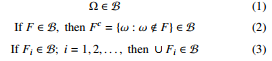
A measurable space is a pair, (Ω, B) consisting of a sample space Ω with a σ-field B of subsets of Ω (also called the event space). A σ-field or σ-algebra B is a collection of subsets of Ω with the following properties:

The type of the measurable space is what differentiates discrete from continuous distributions. More precisely, it is the topology of the sample space. The discrete topology gives rise to discrete probability distributions, and the euclidean topology gives rise to continuous probability distributions.

Let F = {F_i,i = 0,1,2,…,n − 1} be a finite field of sample space Ω, that is, F is a finite collection of sets in Ω that are closed under finite set theoretic operations. To make it more concrete, let us give an example of such a field, which is the power-set of a finite, countable set of atoms (also called categories in the sequel). A set F in F will be called an atom only if its subset is also a field member of itself and the empty set, that is, it cannot be broken up into smaller pieces that are also present in the field. Let A denote a collection of atoms of F . Then, one can show that A consists of exactly all nonempty sets of the form

where F_i^∗ is either F_i or F_i^c. Let us call such sets intersection sets; we observe that any two intersection sets must be disjoint since for at least one i, one intersection set must lie inside F_i and the other within F_i^c. In summary, given any finite field F of the sample space Ω, we can find a unique collection of atoms A of the field such that the sets in A are disjoint, nonempty, and have the space Ω as their union. Thus, A is a partition of Ω. Such a sample space has a discrete topology with the basis given by the set of all atoms A.

Now, we turn our attention to continuous distributions. As already mentioned, the underlying space is the Polish Borel space. An example of such a space, which will be used in this paper, is the

Euclidean space endowed with the Euclidean topology. The basis for the Euclidean topology is the set of all open balls in that space. The Polish space is a complete, separable, metric space. We will explain what the listed properties of the Polish spaces mean.

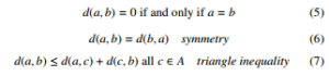
A space is called metric if it is a set A, with elements called points, such that for every pair of points in A, there is an associated non-negative number d(a,b) with the following properties:

A set F is said to be dense in A if every point in A is a point in F or a limit point of F.

A metric space A is called separable if it has a countable dense subset, that is, if there is a discrete set, say B, such that all points in A can be well approximated by points in B. This means that all the points in A are points in B or limits of the points in B. For example, n-tuples of rational numbers are dense in Rⁿ.

A sequence {a_n;n = 0,1,2,… } in A is called a Cauchy sequence if for every  > 0, there is an integer N such that d(a_n,a_m) <  if n ≥ N and m ≥ N. A metric space is complete if every Cauchy sequence converges, that is, if a_n is a Cauchy sequence, then there is a ∈ A for which a = lim_n→∞ a_n.

1.1.2 Probability Spaces

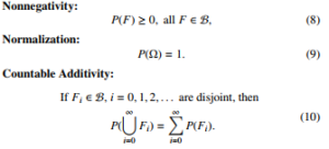
A probability space (Ω, B, P) is a triple consisting of a sample space Ω, a σ-field B of subsets of Ω, and a probability measure P defined on the σ-field; P(F) assigns a real number to every member F of B so that the following conditions are satisfied:

1.1.3 Densities

The probability density function (PDF) is a measure theoretic term defined through the Radon-Nikodym theorem.

A measure m is said to be absolutely continuous with respect to another measure P on the same measurable space, formally m  P, if P(F) = 0 implies m(F) = 0.

Theorem (Radon-Nikodym theorem )

Given the two measures m and P on a measurable space (Ω, F ) such that m  P, there exists a measurable function h : Ω → R with the property that h ≥ 0 such that

The function h is called the Radon-Nikodym derivative or density of m w.r.t. P and is denoted by ^dm_dP . If ^R fdP = 1, then f is called a probability density function.

2. Discrete Distributions

For the statement of all results, as well as notations conventions, we refer the reader to the paper [1]. The results in the article [1] include discussion of the sun rise problem by Pierre-Simon Laplace from the essay [13] and some applications of the theory. We reference the paper [1] in its entirety. Here, only extensions of the material from the paper [1] are included, which have not found place there due to the form of a conference paper. However, for the readers convenience we provide a short summary of the notations used in the derivations:

• K – number of categories, possibly a hidden variable
• M – number of random experiments
• S – the partition, set of all categories
• {p_i}_i∈S – multinomial proportions
• X = {x_i}_(i∈[1,_M],_xi∈_S) – observations from the random experiments
• |A| – cardinality of the set A
• UNIQUE(X) – unique elements in the multiset X
• Z = |UNIQUE(X)| – the diversity index
• P_i = |{x_j : x_j = i}| – counts of the observations

2.0.1    Derivations of the results for the uniform distribution

Assumption of uniform distribution is restrictive. However, it gives initial insight into the problem and, thus, is briefly presented here. As already introduced by X, we denote the sequence of observations. We can show that conditional probability of this sequence given the hypothetical K is equal to:  !          !

It can be seen that the maximum likelihood estimate for the hypothetical number of categories, does not depend on the middle term, which includes the multinomial coefficient. Thus, the estimate can be obtained by,

It is convenient to introduce another quantity, which plays an important role in our theory. This quantity is the generalization coefficient N, which equals by definition:

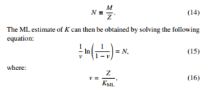
is the fraction of the number of observed categories to the number of all categories. The condition for the likelihood to be monotonically decreasing is as follows:

If this condition holds, the ML estimate for K is equal to Z. The derivations of the above conditions are in place next. First, we note a property that establishes the link with the known in the statistical literature problem of coupon collector [14]:

where one can easily recognize that K × H(K) is the expected number of trials before the coupon collector collects the whole collection. In the above expression, H(K) is the harmonic number, equal by definition:

The main vehicle of the derivation is the following expression that is valid for the harmonic numbers [15]:

where C is the Euler-Mascheroni constant. It can be seen that asymptotically, as K approaches infinity, the terms after the logarithmic term vanish to zero. This leads to the following property:

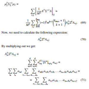
The derivation for the condition (15) begins with taking the logarithm of the considered expression (13):

Suppose, i is a continuous variable, which setting follows from allowing that variable to take on non-integer values. It can be seen that the middle sum does not depend on K; therefore, derivative w.r.t that variable reads:

The last expression allows us to immediately state the (15) and (16).

Equations (15) and (16) allow us to conclude that the sample length needed to learn a given percent of the categories S is a multiple of K. Setting Z = M, we see that, indeed, this (Z = M) is the sufficient and necessary condition for optimal K approaching infinity. This is due to the following identity:

It remains to prove the (17). In this case, the maximum of the likelihood should be attained at K = Z. Thus, we have the following inequality:

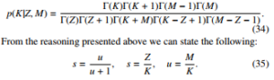
and, after some algebra, we attain at the (17). From the above reasoning all the results pertaining to the discrete, uniform distribution from the paper [1] can be deduced. In Figure 1, we illustrate the dependence of the data amount M needed to learn a given percent

of all categories.

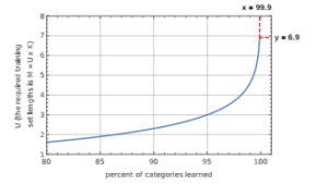
Figure 1: Data amounts requirement to learn a given percent of categories in case of uniform distribution

Next, we discuss the case of the non-uniform distribution, which is more relevant for real-world applications.

2.0.2. Derivations of the results for the non-uniform distribution

The next step will be the derivation of the conditions analogous to that introduced in the previous section, which are distribution-free (we relax the assumption of categories of equal probabilities). The desired effect will be achieved by using the earlier introduced multinomial proportions {p_i}_i∈S . Since we do not impose a constraint on the multinomial proportions, the considered probability function is now in the form, p(X|K, p₁, · · · , p_K) =

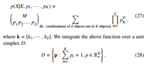
where k = [k₁, · · · ,k_Z]. We integrate the above function over a unit simplex D:

This corresponds to the assumption that all PMFs are equally likely, meaning we assume that we do not know the true PMF and attach to each possible p = [p₁, · · · , p_K] an equal weight (we assume they are equally probable):

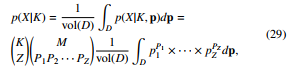
where the expression (29) follows the fact, that the value of the integral does not depend on the choice and order of the probabilities in the monomial integrand. To proceed with the derivation, we compute the integral in (29) using Brion’s formulae; please see [16]:

In light of the above expression, we get,

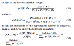
where C is some constant (not to be confused with the EulerMascheroni constant used earlier in this document). Evaluation of (33) yields the following:

Also, all results pertaining to non-uniform distribution, stated in the paper [1], are a consequence of the above reasoning. Based on (35) we can plot the dependence of the amount of data needed to learn given percent of all categories. This dependence is shown in Figure 2.

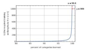
Figure 2: Data amounts requirement to learn a given percent of categories in case of non-uniform distribution

3. Continuous Distributions

The prominent method of density estimation for continuous distribution are Gaussian mixture models (GMM). The GMMs can approximate a PDF given by some training vectors drawn from that PDF. A wide-spread fitting procedure of the GMMs to the given training vectors is based on the Expectation-Maximization (EM) algorithm. Both, the mathematical definition of GMMs and the fitting procedure based on the EM is explained in detail in the book [2]. The neat property of the GMMs is that their expressive power allows modeling any PDF to any accuracy, given enough training vectors are available. However, the traditional fitting procedure is susceptible to overtraining if too many components are chosen. Thus, in this paper, we study a fitting method that does not overfit, and, secondly, allows for the estimation of the number of components given the newly introduced information-theoretic criterion. To reach the goal of formulating the criterion, we first develop a mathematical approach to compute the expected Kullback-Leibler (KL) divergence for the single multivariate Gaussian, whereas the expectation is taken over given number M of samples used to estimate the multivariate Gaussian. In this section, we first develop the theory of expected KL divergence; next, we provide the modified training procedure and end the section with a numerical study.

3.1. Computation of expected Kullback-Leibler divergence

To the best of the authors’ knowledge, the computation of the expected Kullback-Leibler divergence for multivariate Gaussian variables has been never previously explored in the literature. Thus, this paper deals with this problem, which can be formally expressed as,

where p(x) and q(x) are multivariate Gaussians.

The solution to the problem indicated above can be used in the context of the Minimum Description Length (MDL) cf. [17] or Minimum Discrimination Information (MDI), cf. [18]. MDI and MDL principles have been used often for solving computational learning problems (see [19]–[23]).

The well-known result from the statistics is the following formula for the KL divergence between two multivariate Gaussians: Z

p(x)

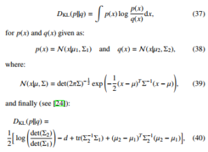
where d is the dimension of PDFs p and q.

Next, let us assume that the positively defined and symmetric Σ₁ is given, µ₁ is a zero vector, and Σ₂ and µ₂ are estimated from samples x_i, where x_i ∼ N(x|µ₁,Σ₁):

where M is the number of samples (length of the observation). We

also assume that Σ₂ is positively definite and thus well-conditioned (otherwise KL divergence would go to infinity). This assumption leads to the requirement that M has to be greater than the dimension of Σ₁ when Σ₂ is non-diagonal.

As already indicated in (36), we are looking for the expectation of the Kullback-Leibler divergence over finite sample:

E_xi∼_p(x) D_KL(p(x)kqˆ(x, x₁, · · · , x_M)),

where p(x) and q(x) are given in (38).

We consider two cases: the first case is when the covariance matrix is diagonal, and the second case, which is a more complicated one, is when the covariance matrix is full.

3.1.1 Diagonal Case

At first, it is worth noticing that the expectation of the KullbackLeibler divergence does not depend on a specific form of the covariance matrix Σ₁. Let us introduce the following substitution:

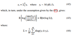
where  denotes the element-wise product, the Hadamard product. It is worth mentioning that we have used the following identity (see [25]):

Since Σ is diagonal and y_i has a zero mean vector, we conclude,

The last expression, which needs to be calculated, is

3.1.2 Non-diagonal Case

In the non-diagonal covariance matrix case, we first introduce the same substitution as in the diagonal case, which is shown in (42):

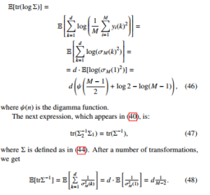
We start by calculating the logarithmic expression, which appears in (40). By using identity in (45), and transforming the expression using (41), as previously, we get,

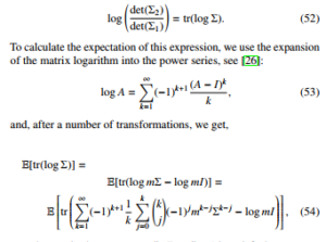
where m is chosen so as to kmΣ − Ik < 1 is satisfied.

We further develop our approximation by introducing the following auxiliary function:

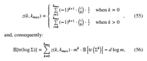
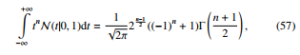
k=0 where d is a dimension of the covariance matrix. To proceed further, we calculate the expectation of tr(Σ^k). It is worth noticing that the integral  !

                                                1                                    n + 1

−∞

vanishes for odd n. At this point, we need to calculate the number of monomials with only even exponents that appear in tr(Σ^k).

Now we can describe the algorithm for calculating the number of such monomials. First, we introduce the following auxiliary matrix:

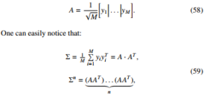
which leads to formula for the specific element, Σⁿ_ij, of the covariance matrix raised to the n-th power:

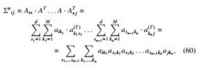
The number of the above configurations with only even exponents is equal to the number of even partitions of 2n. For such a partition, we have to calculate the number of monomials separately. The detailed description of the algorithm for counting monomials is presented in section A. Implementation of the algorithm for counting monomials and computing expected KL divergence is available (see [27]). Below, we have shown examples of the formulas derived by the above-mentioned algorithm, for the power of n = 3, where d is a dimension of the covariance matrix and M is the number of samples used to estimate the matrix:

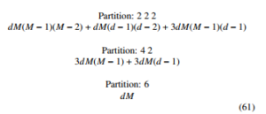
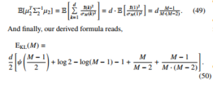
Once we have calculated the number of monomials for each power n, it is relatively easy to calculate the expectation in (56). The second expression, which has to be calculated, is

The next step is to expand inversion of the covariance matrix into the Neumann series (see [28]):

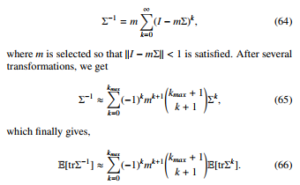
We note that the resulting expression has a similar form to (56), with the difference of the k-dependent expression. The last expression for which the expectation needs be calculated is

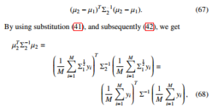
then, given (58), and by expanding the inverse of the covariance matrix as in (64) into the Neumann series, we get: µT2 Σ−21µ2 =

An important observation is in place, namely, the monomials cannot have only even exponents if i , j. This allows us to bring down the calculation of the expectation of the above expression to the expectation of the trace of Σⁿ⁺¹. Thus, finally, we get

Obviously, the algorithm for calculating the above expression is the same as in the case of the two previously examined terms.

3.2. Procedure

Here, we show how to estimate the GMM using the modified training procedure. The introduced procedure solves the problem of overtraining. First, we focus on training the GMM with fixed K – the number of components in the mixture. Based on this development, we formulate a method to select the optimal number of components for a given training set without resorting to the development sets. The classical Expectation-Maximization algorithm, cf. [2], produces in each iteration more and more accurate estimates of the mean vectors, covariance matrices, and weights. We denote the trajectory of these parameters in subsequent iterations as,

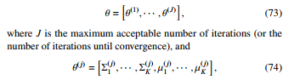
with j the iteration number, Σ_i denoting covariance matrix for the i − th component, µ_i denoting the mean vectors for the i − th component, and K the number of components in the Gaussian mixture. Moreover, we denote ^θ_k^(j) = [Σ⁽_k^j),µ_k^(j)]. To proceed further, we introduce and define some mathematical entities:

• the entropy in nats of the categorical distribution {r_i}_i is defined as H({r_i}) = − ^P_i r_i logr_i
• the kernel width is the effective number of samples used to estimate a given component. Given the samples {x_i}_i^M₌₁, we compute the kernel width, w(θ, {x_i}), also abbreviated by w(θ), using the following set of formulas:

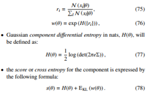
We see that the expression for cross entropy depends only on the observed quantities.

Equipped with the above definitions, we can formulate the algorithm,

Algorithm 1: train GMM Require: starting parameters values θ(0), maximal number of iterations J, initial scores s k , set all weights to ρk = K1 . Ensure: θ(J) and weights {ρk}. 1: for j ∈ [1,…, J] do 2:      compute θ(j) update according to EM (keeping weights unchanged) 3:           for k ∈ [1,…, K] do (j−1) 4:               if s           k                      k                    then 5:                   θk(j) = θk(j−1) (backtracking) 6:              end if 7:         end for 8: end for 9: run few EM updates of weights alone 10: return θ(J) and weights {ρk}

Algorithm 2: train GMM Require: starting parameters values θ(0), maximal number of iterations J, initial scores s k ∞, set all weights to ρk = K1 . Ensure: θ(J) and weights {ρk}. 1: for j ∈ [1,…, J] do 2:      compute θ(j) update according to EM (keeping weights unchanged) 3:           for k ∈ [1,…, K] do (j−1) 4:               if s           k                      k                    then 5:                   θk(j) = θk(j−1) (backtracking) 6:              end if 7:         end for 8: end for 9: run/////////few/////EM/////////updates///of//////////weights///////alone 10: return θ(J) and weights {ρk}

The mechanism behind the algorithm 1 is as follows:

• if the number of components is large in comparison to the number of training vectors, the precision of each component goes up with each iteration until it eventually reaches infinity; this means at the same time, H(θ) goes toward −∞ (in practice, it will stop at a low value due to the constraint we put on the minimal eigenvalue of the covariance matrix)
• the second term in the expression for score, see 78, to the contrary, grows toward +∞ as kernel width approaches dimension of the training vectors d. Thus, even if componenent differential entropy goes toward −∞, the cross entropy has a minimal extreme point and at the very last grows toward +∞.
• thus, the statements from 3-7 in the algorithm 1 prevent the collapse of the components to something resembling a dirac delta
• in effect, the algorithm does not overtrain

We also examine the algorithm 2, which does not run a few EM updates of weights (statement 9 in algorithm 1).

3.2.1 Number of components selection criterion

The cross entropy in 78 is the expression on number of nats needed to code from the component. Based on the cross entropy, we can get the number of bits needed to code with given fidelity using the Shannon-Lower-Bound [29].

Given the component weights {ρ_k}_k^K₌₁, the average number of nats needed to code from the GMM modeled source PDF is equal to

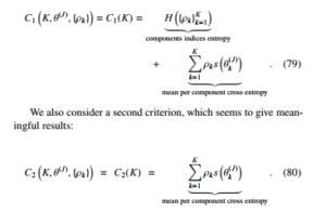
mean per component cross entropy

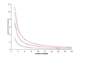
Figure 3: Comparison of the empirically and analytically obtained expectation of the KL divergence for Gaussians with the diagonal covariance matrices. Dashed lines represent the Monte Carlo result. Dimensions of covariance matrices from the beginning of the coordinate axes: 3, 7, and 11, respectively.

To find the optimal number of components K (which minimizes the average number of nats needed to code from the source), we proceed as follows:

• we swap the K from 1 to M
• for each K we run the algorithm 1 or 2.
• we smooth with smoothing splines, see [30], the resulting curve C_∗(K), obtaining a smoothed curve C˜_∗(K)
• we select Kˆ for which C˜_∗(Kˆ) attains minimum and returns the optimal number of components.

Above, the asterisk means either 1 or 2.

3.3. Numerical experiments

3.3.1 Expected Kullback-Leibler Divergence

In this section, the comparison our analytical results with the MonteCarlo obtained curves of expected Kullback-Leibler divergence will be presented. First, the results for the diagonal covariance matrix will be shown in Figure 3.

As can be seen, the analytical expectation shows high accuracy for the diagonal covariance matrices.

The results are a bit worse for the non-diagonal matrix. The following issues affected the accuracy of the result:

• the calculation of the higher degree series expansions was too hard as the computation of the number of even exponent monomials grew exponentially with n. We were able to compute the number of monomials for n as high as eight (the formulas for n = 8 when written on A4 page taking 44000 rows).
• The Monte-Carlo curves on the left are sensitive to the threshold for the detection of the semi-definiteness of the matrices. It sometimes happens that one of the eigenvalues of the covariance matrix is very small. Then value of term trΣ⁻¹ grows enormously. It is clear that the result depends on the choice of the threshold.

Figure 4 depicts the results for non-diagonal covariance matrices. To obtain the plot, we rejected matrices with the smallest eigenvalue less than 0.01 (which is around  of the largest eigenvalue).

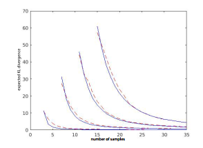
Figure 4: Comparison of empirically and analytically obtained expectation of the KL divergence for Gaussians with the non-diagonal covariance matrices. Dashed lines represent the Monte Carlo estimation. Dimensions of covariance matrices from the beginning of the coordinate axes: 3, 7, 11, and 15, respectively.

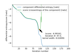
Figure 5: Illustration of the overtraining prevention mechanism. Plot shows that score prevents the overtraining, differential entropy of the Gausssian component goes down and the score starts increasing after kernel width exceeds 8 training points

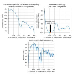
Figure 6: Results of the algorithm 1 for d = 2

3.3.2 Overtraining Prevention Mechanism

Here, we present a drawing (Figure 5) showing the trajectory of the score and component differential entropy. The plot has been obtained by by recording the parameters for subsequent iterations for one chosen component of the GMM. We see that the score attains minimum but component differential entropy goes to −∞. This allows to use the backtracking procedure present in algorithms 1 and 2.

3.3.3 Numerical Analysis of the Number of Components Selection Criteria

All numerical experiments of this section has been carried out using the Line Spectral Frequencies (LSF) as the data to which the GMMs are fitted. The LSFs were computed from the LibriSpeech database. In all subsequent experiments the training set length M equals 1000.

First, the workings of the algorithm 1 will be presented. The Figure 6 shows the criteria C₁ and C₂ and the components indices entropy on pictures from left to right and from top to bottom, respectively. We see erratic behaviour of the components indices entropy that falls down, meaning it silences some components by driving some weights to zero. The criterion C₁ suggests that the optimal number of components is > 500, what is unlikely and probably caused by silencing of some components by zero weights. The C₂ criterion, instead, gives a sensible result. We see that for algorithm 2, selected by the C₂ criterion, number of components is similar.

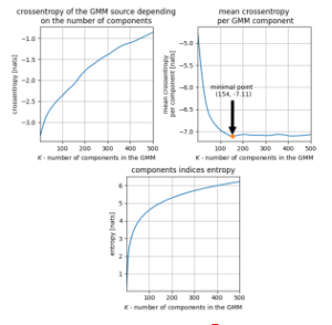
Figure 7: Results of the algorithm 2 for d = 2

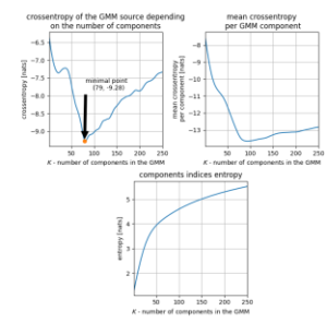
Figure 8: Results of the algorithm 2 for d = 4

As the second example, we show the workings of the algorithm 2. The plots in Figure 7 show the same curves as in the case of the Figure 6 (see previous paragraph). The C₁ criterion points as the optimal number of components exactly one component, that is, a single Gaussian. Above K = 1, the components indices entropy penalizes the score to the extent that the score curve is monotonically increasing. Another optimal number of components is suggested by C₂. We computed the GMMs for the number of components selected using the C₂ criterion, for which the contour plots are shown on Figure 10. We see that the GMM is tightly fitted to the data for the selection criterion C₂. However, the composite criterion C₁ suggests a single component, which seems to by trivial, but still optimal, as indicated by the methodology proposed.

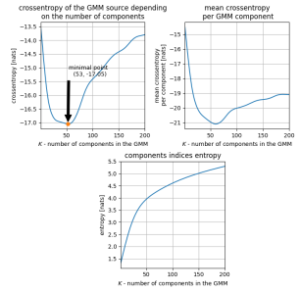
Figure 9: Results of the algorithm 2 for d = 8

As the third example, we show the working of the algorithm 2 for the problem dimension d = 4 (first four line spectral frequencies). In this case, the criterion C₁ returns trustworthy results, the minimum on the C₁ curve is clearly noticeable. The returned result is sensible and indicates that for d = 4, the training vectors distribution needs more components to be modeled accurately; the distribution is probably far from Gaussian. The curves are presented in Figure 8. This experiment is an indication that the proposed methodology is sound. To make the evidence even stronger we present more experiments for dimensions d = 8, Figure 9, and d = 16, Figure 12. As expected the optimal number of components decreases with the dimension of the problem. This is to maintain proper generalization.

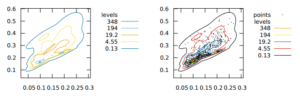
Figure 11: GMM fitted using traditional EM algorithm with number of components selected using tuning on the development set

The last result shows the behavior of the classical number of components selection criterion, that is the maximization of the likelihood on the development set. For this experiment, from 1000 samples of the training set, we excluded 100 samples as the development set. In Figure 13, we show the plot of the log-likelihood on the development set as a function of the number of components. It is evident that the plot is quite erratic of what decreases trust in this method of selection of the number of components. The results can be made more stable if we allow the development set to be larger. Such a measure will come at the cost of reducing the number of training points. Here, our proposed method shows the advantage of not using development sets. The contour plots for the GMM fitted using traditional method with the number of components tuned on the development set are shown in Figure 11.

4. Conclusions

In this paper, the theory of both discrete and continuous distribution with unknown number of components has been developed. The measure theoretic reason for the inherent similarity between PMFs and PDFs, with the difference in the structure of the underlying sample space, has been given. The difference causes the two distribution categories to be treated with much different mathematical tools. The main result of the paper are the means and methods of computing the number of components, that is, the number of categories in the PMF case and the number of Gaussian components in the GMM modeling in a PDF case, which is given implicitly in terms of its realizations.

Development of the theory required considering the expected Kullback-Leibler divergence – a difficult problem on its own rights. Especially, the algorithm for counting monomials with only even exponents in the expression for a trace of a matrix raised to a power has been developed. This algorithm allows to compute certain integrals analytically without resorting to the Monte-Carlo experiments. This algorithm can also be of interest on its own rights.

We believe that the theory presented in this paper will find many practical applications in diverse fields of science, technology, and engineering as a convenient tool of data analysis.

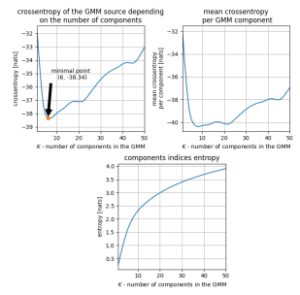
Figure 12: Results of the algorithm 2 for d = 16

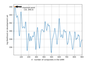
Figure 13: Results of the traditional EM algorithm d = 2

1. M. Kuropatwin´ski, “Estimation of Quantities Related to the Multinomial Dis- tribution with Unknown Number of Categories,” in 2019 Signal Processing Symposium (SPSympo), 277–281, 2019, doi:10.1109/sps.2019.8881992.
2. C. M. Bishop, Pattern recognition and machine learning, Springer, 2006.
3. R. M. Gray, Source coding theory, Springer, 2012.
4. R. M. Gray, “Gauss Mixture Vector Quantization,” in IEEE International Conference on Acoustics, Speech, and Signal Processing, 1769–1772, 2001, doi:10.1109/icassp.2001.941283.
5. S. Young, G. Evermann, M. Gales, T. Hain, D. Kershaw, X. Liu, G. Moore,
   J. Odell, D. Ollason, D. Povey, et al., The HTK book, Cambridge University Engineering Department, 2002.
6. D. A. Reynolds, T. F. Quatieri, R. B. Dunn, “Speaker verification using adapted Gaussian mixture models,” Digital Signal Processing, 10(1), 19–41, 2000, doi:10.1006/dspr.1999.0361.
7. H. Permuter, J. Francos, I. Jermyn, “A study of Gaussian mixture models of color and texture features for image classification and segmentation,” Pattern Recognition, 39(4), 695–706, 2006, doi:10.1016/j.patcog.2005.10.028.
8. A. Kundu, S. Chatterjee, A. S. Murthy, T. Sreenivas, “GMM Based Bayesian Approach To Speech Enhancement in Signal/Transform Domain,” in 2008 IEEE International Conference on Acoustics, Speech and Signal Processing, 4893–4896, 2008, doi:10.1109/icassp.2008.4518754.
9. M. Nilsson, H. Gustaftson, S. V. Andersen, W. B. Kleijn, “Gaussian Mixture Model Based Mutual Information Estimation Between Frequency Bands in Speech,” in 2002 IEEE International Conference on Acoustics, Speech, and Signal Processing, 525–528, 2002, doi:10.1109/icassp.2002.1005792.
10. B. W. Silverman, Density estimation for statistics and data analysis, CRC Press, 1986.
11. L. Devroye, G. Lugosi, Combinatorial methods in density estimation, Springer, 2012.
12. R. M. Gray, Probability, random processes, and ergodic properties, Springer, 1988.
13. P.-S. Laplace, Philosophical essay on probabilities, Springer, 1998.
14. P. Flajolet, D. Gardy, L. Thimonier, “Birthday paradox, coupon collectors, caching algorithms and self-organizing search,” Discrete Applied Mathematics, 39, 207–229, 1992, doi:10.1016/0166-218x(92)90177-c.
15. S. Gradshteyn, I. Ryzhik, Table of integrals, series, and products, Academic Press, 2014.
16. V. Baldoni, N. Berline, J. De Loera, M. Ko¨ppe, M. Vergne, “How to integrate a polynomial over a simplex,” Mathematics of Computation, 80(273), 297–325, 2011, doi:10.1090/s0025-5718-2010-02378-6.
17. J. Rissanen, “Modeling by shortest data description,” Automatica, 14(5), 465– 471, 1978, doi:10.1016/0005-1098(78)90005-5.
18. S. Kullback, Information theory and statistics, Courier Corporation, 1997.
19. R. H. Davies, C. J. Twining, T. F. Cootes, J. C. Waterton, C. J. Tay- lor, “A minimum description length approach to statistical shape model- ing,” IEEE Transactions on Medical Imaging, 21(5), 525–537, 2002, doi: 10.1109/tmi.2002.1009388.
20. R. M. Gray, J. C. Young, A. K. Aiyer, “Minimum Discrimination Infor- mation Clustering: Modeling and Quantization with Gauss Mixtures,” in 2001 International Conference on Image Processing, 14–17, 2001, doi: 10.1109/icip.2001.958039.
21. M. H. Hansen, B. Yu, “Model selection and the principle of minimum descrip- tion length,” Journal of the American Statistical Association, 96(454), 746–774, 2001, doi:10.1198/016214501753168398.
22. Y. Ephraim, A. Dembo, L. R. Rabiner, “A minimum discrimination information approach for hidden Markov modeling,” IEEE Transactions on Information Theory, 35(5), 1001–1013, 1989, doi:10.1109/18.42209.
23. R. M. Gray, A. Gray, G. Rebolledo, J. Shore, “Rate-distortion speech coding with a minimum discrimination information distortion measure,” IEEE Trans- actions on Information Theory, 27(6), 708–721, 1981, doi:10.1109/tit.1981. 1056410.
24. J. Duchi, “Derivations for Linear Algebra and Optimization,” Technical report, University of California at Berkeley, 2007.
25. C. S. Withers, S. Nadarajah, “log det A = tr log A,” International Journal of Mathematical Education in Science and Technology, 41(8), 1121–1124, 2010, doi:10.1080/0020739x.2010.500700.
26. B. Hall, Lie groups, Lie algebras, and representations: An elementary introduc- tion, Springer, 2015.
27. L. Sikorski, M. Kuropatwin´ski, “Counting Monomials Algorithm,” https://www.codeocean.com/, 2019, doi:10.24433/CO.3748956.v1.
28. D. Zhu, B. Li, P. Liang, “On the Matrix Inversion Approximation Based on Neu- mann Series in Massive MIMO Systems,” in IEEE International Conference on Communications (ICC), 1763–1769, 2015, doi:10.1109/icc.2015.7248580.
29. T. Berger, Rate distortion theory: A mathematical basis for data compression, Prentice-Hall, 1971.
30. C. De Boor, A practical guide to splines, Springer, 1978.

(Click Here)

(Click Here)