1. Introduction

Acoustic emission (AE) in solid bodies is elastic oscillations occurring in the result of dislocation changes in a medium. In such a case, the characteristics of generated pulse emission are directly associated with plastic process features. That determines the interest in the emission investigation with the aim to develop methods for medium acoustic diagnostics.

AE is applied for different problems of diagnosis in seismology, geophysics as well as in non-destructive testing of objects and materials in industry. At the beginning of the XXI century it was shown that acoustic emission anomalies are observed before strong earthquakes and can be consider as their operative precursors [1-3]. In further investigations [4, 5] the nature of generation of pre-seismic acoustic anomalies and the features of their manifestations were considered. In the course of the research carried out at IKIR FEB RAS, it was shown that these anomalies are generated by the change of geomechanics stress field in earthquake preparation zone and appear as the result of the transformation, stress – near-surface rock deformation [6, 7]. The peculiarity of anomaly manifestation is geoacoustic emission intensity increase in the frequency range from hundreds of hertz to the first tens of kilohertz. It usually lasts for to several hours and occurs 1–3 days before an earthquake.

Statistics of pre-seismic acoustic anomaly observations in a seismically active region of Kamchatka peninsula, which is a part of the Pacific Ring of Fire, shows high efficiency and prospectivity of AE method to forecast catastrophic earthquakes [6]. Detailed analysis of AE signals shows that they a represented by a sequence of relaxation oscillation pulses with steep edge and smooth drop of different frequency filling [6]. In these circumstances, both separate pulses and their groups with significant overlapping are observed. In case of intensive emission, pulses merge into a continuous signal.

During a background (seismically calm) period, acoustic pulses with the repetition frequency within 0.1–0.5 pulses per a second are usually observed. During the increase of stress and of rock deformation velocity before an earthquake, both pulse amplitude and their number per a time unit grow. Pulse repetition frequency reaches the value of tens and even hundreds per a second [6].

At the present time one of the main and still unsolved problems is automation of search and operative detection of AE pre-seismic anomalies. Application of popular (widely spread in the world) methods for data analysis becomes complicated by several reasons, they are:

• wide dynamic range of recorded data is associated with great volumes of recorded information requiring special methods for storage, transfer, processing and analysis;
• strong irregularity of natural mediums and bad propagation of elastic oscillation causes signal significant distortion and attenuation which limits the capabilities
  of investigation methods;
• strong noisiness both by natural and industrial noises makes the analysis of inner (morphological) structure
  of AE pulses more complicated;
• wide variety of signal waveforms complicates the problem of classification and requires analysis methods adapting for a given signal.

The paper proposes a new approach to analyze and classify rock acoustic emission signals in order to identify AE pre-seismic anomalies. The approach is based on the description of acoustic pulses from which a signal alphabet is formed. Then the changes of alphabet parameters of signal subsequent fragments are studied.

2. AE signal model

In a general case, acoustic emission signals can be represented by a classical adaptive model, i.e. as a sum of noise ε(t) and some function s(t), the analytical expression of which is unknown,

where ε(t) describes nonstationary background noise containing noises of natural and artificial origin and s(t) is a “useful” AE signal. It is a flux of pulses of different waveform, amplitude and frequency. Moreover, we accept the following constraint ||s(t)|| > ||ε(t)||. Figure 1 illustrates an example of AE signal.

Within the framework of the proposed approach, pulses
of a “useful” signal s(t) can be described by the means of their singular points. As it is known from the functional analysis theory, when there are no fractures of the first and of the second kind, these points coincide with local extrema and local inflections. It is assumed that signal function intermediate values lying between the singular points are less informative and may be neglected in the course of the analysis.

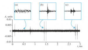
Figure 1: Acoustic emission signal: (a) – noise, (b), (c) – pulses

In order to understand the essence of further transformations, we consider an acoustic emission pulse signal (its graph is illustrated in Figure 2). We fix the values pulse local extreme amplitudes {a_i} = a₀, a₁, …, a_N and the time intervals between neighboring extrema {τ_i} = τ₀, τ₁, …, τ_N-1. On the basis of these values we create a matrix of mutual relation of the fixed values (2). Matrices of A and T relation reflect pulse amplitude-phase structure. They characterize the positions of local extrema relatively each other and can be considered as a pulse model.

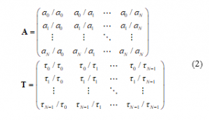
We should note that if one knows any one value a_i, any one value t_i and the relational matrix (2), it is possible to recover the initial waveform of a pulse more or less without loss.

To compose signal symbol description, the obtained pulse diversity is classified by comparing the relational matrices (2), i.e. based on the pulse waveform similarity criterion. However, such selection should take into account two key points: firstly, amplitude attenuation and phase distortions of acoustic pulses occurring during the propagation from a source to a receiver point; secondly, the distortions caused by the interference of additive noise on pulse waveforms at a receiver point. These problems inevitably result in significant increase of the number of pulse classes (redundant classification). The following transformations and computing operations allow us to solve, to a large extent, the problems arising during the classification.

When analyzing a pulse waveform, signal function numerical values at singular points often do not play the major role. In a greater degree, to detect a pulse waveform, mutual position of these points is important [8]. In the framework of the applied approach, search for the differences in the observed pulse waveforms is of the main interest. Thus, relational matrices can be reduced to matrices of rank relation. In order to do that,it would be enough to transform matrices (2) into binary ones according to the following rule:

Figure 2: Local extrema of AE pulse

where r_i,j is the result of comparison of the i-th and j-th vales of extreme amplitudes; w_i,j is the result of comparison of the i-th and j-th values of the intervals between the extrema. We create binary matrices of the comparison (3) results for amplitudes R and time intervals W separately.

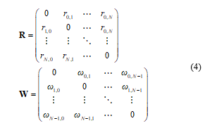
The obtained binary square matrices R and W (4) of the sizes N+1 and N, respectively (intervals between local extrema are less by 1) have redundant character since, owing to inequality asymmetry (if a > b, then b ≤ a), we have r_i,j = Ør_j.i and ω_i,j = Øω_j,i, and all the elements lying on the main diagonal are equal to 0. In order to represent the pulse waveform more compactly, we join significant elements of both matrices. Transform the matrices R and W into upper triangular ones zeroing the redundant elements according to (5)

As the result we obtain triangular binary matrices R_Δ and W_Δ (6).

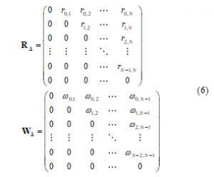
We reduce the matrix R_Δ size to the value N by removing zero elements of the lower line and the left column. We make transposition operation of the matrix W_Δ and as the result obtain the matrix W_Δ^T. After summing up the matrices R_Δ and W_Δ^T, we obtain a square binary matrix D of size N (7). It can be used as a model of pulse amplitude-phase structure.

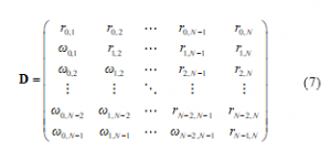
We call (7) a pulse descriptive matrix.  An example of a pulse and its descriptive matrix are illustrated in Figure 3.

Figure 3: Representation of a pulse by descriptive matrix: (a) – pulse with detected extrema; (b) – pulse descriptive matrix

Descriptive matrices have invariant character under time and amplitude transformations that is proved by the following properties:

• invariance under time compression or expansion (if k> 0 and τ_i > τ_j, then τ_i ∙ k > τ_j ∙ k);
• invariance under amplitude compression or expansion (if k> 0 and a_i > a_j, then a_i ∙ k > a_j ∙ k).

The invariance is retained, if the coefficient k is substituted by any monotone positive function f(x) > 0. Attenuation processes and nonlinear amplitude-phase distortions, changing AE pulse signal waveforms during its propagation in heterogeneous anisotropic mediums from a source to a receiver, have the character of monotone functions in the majority of practical cases. Thus, descriptive matrix invariance is of great importance when creating algorithms for identification and classification of acoustic emission pulses.

3. Model adequacy

To verify the proposed model adequacy, we generated two artificial AE signals.

It was shown in the paper [9] that AE typical pulses are described by modulated Berlage functions with a reasonable degree of accuracy

where A is the pulse amplitude; t is the time, 0 ≤ t ≤ t_end; p_max is the pulse envelope maximum position defined relating to t_end; n(p_max) is the minimum value of the parameter affecting pulse envelope slope which is chosen so that u(p_max · t_end) ≤ 0.05·u(t_end); Δ is the coefficient of pulse envelope slope variation, the more Δ value is, the steeper the envelope is, Δ > 1; f is the pulse modulation frequency; φ₀ is the initial phase. To obtain different pulse waveforms, the parameter values p_max, Δ, t_end, f, φ₀ vary.

The first artificial signal (Figure 4a) contains five pulsesof similar waveform and the second one contains five pulsesof different waveform (Figure 4b). As long as the model should be invariant under amplitude and time transformations of the signal, the length and the amplitude of each pulse were drawn at random. Instead of the frequency f, the number of periods k on the time interval from 0 to t_end was defined. Parameters of the generated pulses are listed in Table 1.

Table 1: Parameters of test pulses

Wave-form	Number of periods, k	Maximum position, pmax	Steepness, Δ	Initial phase, φ0
I	10	0.2	1.5	0
II	5	0.1	1.2	0
III	15	0.25	2	0
IV	11	0.01	1	π/3
V	20	0.4	1.5	0

Signal graphs and modeling results are illustrated in Figure 4a–b. Pulses having similar descriptive matrices are shown by the same color. Thus, application of the proposed model allowed us to determine correctly the similarity/difference of pulse waveforms. We should note that the pulses of the first signal have different frequency-time structures (Figure 4c), and would be attributed to different classes when applying frequency-time methods. Pulses of the second signal have the same frequency (Figure 4d), but different waveforms and would be attributed to the same class when applying frequency-time methods.

Figure 5 shows the real AE signal containing five pulses. Three pulse waveforms are distinguished visually. The suggested model describes real signals adequately. Pulses of the same waveform have similar descriptive matrices.

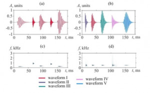
Figure 4: Modeling results for two signals. Pulses described by the same descriptive matrix are of the same color: (a) – signal containing five pulses of the same waveform; (b) – signal containing five pulses of different waveform; (с) – Wigner-Ville transformations of the first signal pulses; (d) – Wigner-Ville transformations of the second signal pulses

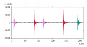
Figure 5: Modeling results for real AE signal. Pulses described by similar descriptive matrices are of the same color

In the considered examples we analyze the signals in which noises are either absent or insignificant. Real AE signals often contain noises of artificial and natural origin, thus perturbing a signal. Distortion may result in a gap, false detection or amplitude change of some extrema. Then the size and some elements of pulse descriptive matrices differ (Figure 6).

4. Classification of pulse diversity

We define initial conditions for classification. We put bounds on the size of descriptive matrices detected during the analysis by the values N_min and N_max from the bottom and from the top, respectively. Analysis epoch is the length of the time window in which an AE signal is observed. In practice, this index should provide formation of stable classes. N_min is determined by the minimum number of oscillations during pulse duration and cannot be set less than 3. N_max is defined according to the capabilities of a computing device and the maximum run-time.

Pulses are classified accorded to the results of calculation of descriptive matrix similarity coefficient. First, we restrict ourselves to descriptive matrices of the same size. In order to do that we divide descriptive matrices into groups D^(Z) of matrices of the same size Z, N_min < Z < N_max.

For the two descriptive matrices of the same size D₁^(Z) and D₂^(Z) the similarity coefficient g(D₁^(Z), D₂^(Z)) is determined as a ratio of elements, coinciding in value and taking the same positions, to the total number of elements in the matrix. In case of exact identity, the similarity coefficient is 1.

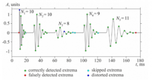
Figure 6: Examples of errors occurring during extreme detection

where #(condition) is the operator for calculation of the number of elements satisfying the condition, d_1ij are the elements of the matrix D₁^(Z), d_2ij are the elements of the matrix D₂^(Z).

The calculated similarity coefficient g(D₁^(Z), D₂^(Z)) is compared with the selected threshold value G₀ (it is chosen empirically). If

then the pulses described by D₁^(Z) and D₂^(Z) belong to the same class.

Classification is the comparison of descriptive matrices of the same size and selection of the empirical threshold G₀ (0 < G₀ ≤ 1) with which the similarity coefficient (9) is compared.

The possibility that two pulses of the same source will have exactly the same number of local extrema is very low. So, the obtained classification is too restrictive. Thus, we developed a procedure to compare descriptive matrices of different sizes. It takes into account false extrema or gaps of some extrema and allows us to reduce the number of detected classes. However, when descriptive matrix sizes are widely scattered, they are compared in erratic manner that may cause random merging of classes described by descriptive matrices of smaller sizes. We put bounds on the possibility for merging of descriptive matrices of smaller sizes by the threshold coefficient S₀:

where N_L and N_M are the sizes of smaller and larger descriptive matrices, respectively, S₀ is the empirically defined threshold.

Assume that there are two descriptive matrices D₁ and D₂ of the sizes N₁ and N₂, respectively (N₁ ≥ N₂). If N₂/N₁ ≥ S₀ (N = S₀ · N₁), then the matrices are comparable. For the meaningful comparison, the matrices D₁ and D₂ are matched so that the latest N elements of the main diagonal D₂ are overlapped on the first N elements of the main diagonal D₁. Then we calculate the similarity coefficient (9) of matrices of size N in the domain bounded by the intersection. Elements are further compared after D₂ shift along the main diagonal D₁. The similarity coefficient (9) is calculated for each subsequent shift so far as the matrices in the domain bounded by the intersection have the size of not less than N (Figure 7). The comparison result is the maximum value of the similarity coefficient.

If the maximum similarity coefficient (9) exceeds the empirically defined threshold G₀ or is equal to it, the decision on sufficient closeness of descriptive matrices of compared pulses is made. In this case, the pulse with descriptive matrix of the smaller size is included into the class described by larger-size descriptive matrix (larger object absorbs a smaller one).

Figure 7: Comparison of descriptive matrices of sizes 6 and 5

In the result of classification many classes are formed. Each of them unites the pulses close in amplitude-phase structure with the accuracy up to the values determined by the coefficients G₀ and S₀. Each class can be considered as some symbol and the whole set of obtained symbols composes a signal alphabet.

In order to estimate the classification algorithm noise immunity for different values of the thresholds G₀ and S₀, we realized a simulation experiment. We processed the data containing 100 pulses of similar waveform (the alphabet cardinality is 1 symbol) with signal/noise ratio (SNR) from ¥ to 2.7 dB.

At the first stage of the experiment we compared the descriptive matrices with sizes differing by less than 30% (S₀ ≥ 0.7). Similarity coefficient threshold was chosen to be G₀ = 1 (case when a matrix of smaller size is the sub-matrix of a larger-size matrix).

Figure 8 shows the dependences of alphabet cardinality on SNR for different values of the coefficient S₀ (0.7–1). Insignificant difference of the graphs proves that descriptive matrix element values significantly depend on local influence of noise on pulse waveform and are weakly sensitive to changes in the threshold S₀ at a high value G₀. When SNR values are less than 30 dB, the classification does not work since matrices do not match with 100% agreement (G₀ = 1).

Figure 8: Dependence of alphabet cardinality on SNR for different values of the threshold S₀ (0.7–1) and for a fixed valued of the threshold G₀ =1

At the next stage of the computational experiment, we investigated class formation during threshold G₀ changes (from 0.6 to 0.9). In this case, matrices of the same size (S₀ = 1) were compared. The results of the second stage of the computational experiment are illustrated in Figure 9. The graphs show that decrease of the threshold G₀ causes significant reduction of alphabet cardinality. Moreover, the number of detected classes reduces with G₀ decrease.

Figure 9: Dependences of alphabet cardinality on SNR for different values of the threshold G₀ (0.6–0.9) and for a fixed value of the threshold S₀ = 1

At the third stage of the computational experiment we investigated the dependence of alphabet cardinality on SNR for S₀ = 0.7 and different values of G₀. The results are shown in Figure 10.

The experiment shows that the classification method is nonlinearly sensitive to the choice of threshold functions of G₀ and S₀: decrease of S₀ causes pulse redistribution into classes with larger-size descriptive matrices and decrease of G₀ makes it possible to compact classes. Based on the experiment results, the recommended values of the thresholds S₀ (from 0.6 to 0.9) and G₀ (from 0.7 to 0.9) were selected.

As long as the developed method of classification is expectedly sensitive to the performance quality of the algorithms for pulse detection and noise reduction, one of the important tasks in AE signal investigation is the improvement of methods for signal pre-processing.

Classical digital filtration, empirical mode decomposition (EMD), and wavelet filtration were considered as methods of noise reduction and detection of signal useful component. Digital filtration was not used because the AE pulses have short duration (100–400 samples per pulse). Problem of mode functions selection complicated the usage of EMD for signal denoising (for example, in [10]), since rejected modes are different for different pulses. So, the authors chose wavelet filtration technology with adaptive threshold scheme. Wavelets are widely used in various signal processing tasks [11], in particular in noise reduction tasks [12, 13]. Denoising has three stages: direct wavelet transforms, application of a selected threshold scheme to every detailing component, inverse wavelet transforms. In order to choose a wavelet family, a threshold scheme and an algorithm for calculating threshold value, a computational experiment was carried out on model and real AE signals. The best results were obtained applying fourth-order symlets (maximum possible level of decomposition), median threshold scheme and empirical Bayes rule to calculate the threshold value [14, 15]. The selected wavelet filtration method allows us to increase the signal-to-noise ratio by about 9 dB, on the condition that initial SNR is 8.9 dB.

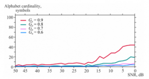
Figure 10: Dependences of alphabet cardinality on SNR for different values of the threshold G₀ (0.6–0.9) and for a fixed value of S₀ = 0.7

Figure 11a–b illustrates the process of detection of local extrema in a noised pulse and in a pulse with additive noise. Figure 11c shows how the wavelet filtering algorithm recovers the waveform of a perturbed signal.

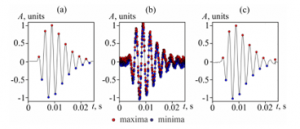
Figure 11: Noise effect on detection of local extrema: (a) – initial pulse; (b) – pulse with overlapped white noise, SNR = 12.4 dB; (c) – pulse denoised by wavelet filtration, SNR = 22.7 dB

Application of wavelet filtering with adaptive threshold schemes allows us to apply the proposed methods of analysis to perturbed and noisy signals.

Figure 12 illustrates the results of classification of model signal pulses with the signal/noise ratio of 8.9 dB. The signal contains 50 Berlage pulses described by three waveforms the parameters of which are listed in Table 3. Before being classified, each detected pulse was denoised by the selected method of wavelet filtering (after wavelet filtration, the SNR of a single pulse is about 20 dB). When constructing descriptive matrices, we did not take into account the extrema the amplitudes of which were less than 15% from the maximum one. Classification algorithm thresholds were selected as S₀ = 0.6 and G₀ = 0.7. For a noisy signal (Figure 12а) we succeeded to define correctly the number of classes and to structure the pulses into classes (Figure 12b). In the course of multiple repetition of the experiment it was discovered that the obtained structuring into the classes is stable to the changes of initial conditions of white noise generator.

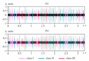
Figure 12: Classification results: (a) – signal with overlapped white noise and initial structuring into classes; (b) – classification of S₀ = 0.6, G₀ = 0.7; 3 classes were defined

Table 2: Waveform parameters

Class	Number of periods, k	Maximum position, pmax	Steepness, Δ	Initial phase, φ0
I	7	0.05	1.1	0
II	20	0.35	3	π/3
III	40	0.2	2	π/2

The proposed algorithm classifies correctly 78% of pulses, on the conditions that thresholds are selected as S₀ = 0.6, G₀ = 0.7 and SNR is 8.9 dB before wavelet denoising. This estimate is based on the results of 100 experiments.

Efficiency of the proposed classification method can be estimated by a contraction coefficient

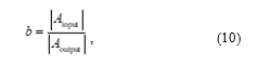
where |A_input| is the alphabet cardinality (number of pulses) before classification, |A_output| is the cardinality of the alphabet obtained as the result of classification.

Table 3 illustrates the classification results for 12 files containing 15-minute records of AE signals from IKIR FEB RAS archive data for January 1, 2018. The classification was carried out with the coefficients G₀ = 0.8, S₀ = 0.8.

As the result of further processing of AE data for the period 2016-2019, it was determined that contraction coefficient (10) varies from 50 to 200.

The developed methods of pulse description and classification were realized in the form of software. Preprocessing procedures such as centering, normalization, and noise reduction were performed by MATLAB system.

Table 3: Classification results

File number	Alphabet cardinality, |Ainput|	Alphabet cardinality, |Aoutput|	Contraction coefficient, b
1	2864	37	77.4
2	3233	36	89.8
3	3581	46	77.8
4	3986	43	92.6
5	4593	45	102.0
6	3132	46	68.0
7	3778	43	87.9
8	4424	38	116.4
9	4836	36	134.3
10	3968	39	107.7
11	4734	36	131.5
12	3475	44	78.9

5. Examples of identification of pre-seismic AE anomalies

The developed method of classification was realized in the form of an application program. It was used to process and to analyze acoustic emission signals recorded in 2016–2019 at “Karymshina” site of IKIR FEB RAS (52.83º N, 158.13º E). AE signals are stored in the database in the form of 15-minute sound files (WAVE format). In the course of processing of each file, signal alphabet was constructed. Then alphabet symbols were ranked according to the size of their descriptive matrices and frequency (number of pulses described by the symbols).

Based on the conception of the relation of AE signal parameters with the state of a system generating a signal, we should analyze quantitative and qualitative parameters of symbol description of a signal for different time periods (from a day to a year) and to compare the defined anomalies with occurred earthquakes according to the data of regional seismic catalogue (Kamchatka Branch of the FRC GS RAS, Earthquake Catalogue for Kamchatka and Kuril Islands (1962 – present time), http://sdis.emsd.ru/info/earthquakes/catalogue.php).

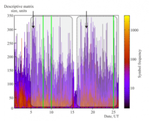
Figure 13: Anomalous dynamics of AE signal alphabet in October 2017

In order make the analysis, alphabets of each 15-minute AE signal were formed. Then three-dimensional images of a special type were drawn. Descriptive matrix size was measured on the vertical axis. Time (with 15-minute step) was measured on the horizontal axis. Color denotes symbol frequency.

Examples of anomalies observed 1–12 days before earthquakes and 1–6 days after earthquakes are illustrated in Figures 13–15.

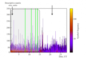
Figure 14: Anomalous dynamics of AE signal alphabet in February 2019

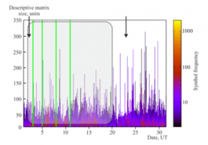
Figure 15: Anomalous dynamics of AE signal alphabet in October 2019

Anomaly peaks in the Figures are marked by black arrows. Green lines indicate earthquake times. These anomalies are alphabet content redistribution in favor of the symbols described by larger-size descriptive matrices (up to 350 extrema). Simultaneously with that the number of such symbols increases. Alphabet cardinality also grows from 20 to 150. Assumed areas of anomalies associated with earthquakes are marked by rounded rectangles. Short-term changes of alphabet content (less than 305 peaks) were not taken into consideration.

We should note that not all the analyzed AE anomalies in the form of redistribution of alphabet symbol frequency are associated with earthquake preparation processes. In the experiment the acoustic emission is recorded in sedimentary rocks and is a sensitive indicator of their stress-deformed state. Both global tectonic processes (for example, earthquake preparation) and local deformations, associated with the impact of different natural factors, may influence that state. Thus, not all the recorded AE anomalies are pre-seismic.

Figures 13–15 illustrate examples of AE anomalies observed during the periods when earthquakes occurred quite rarely, from one to four strong events per a month. Such a choice allows us to demonstrate the relation of detected anomalies with earthquakes. When earthquakes repeat quite frequently, the anomalous behavior is not so clear that may be explained by overlapping of fragments of evoked anomalous effects. Example of such behavior of alphabet content dynamics is shown in Figure 16.

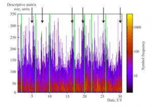
Figure 16: Anomalous dynamics of AE signal alphabet in April 2017

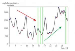
Figure 17: Graphs of AE signal alphabet cardinality dynamics in September 2017

Further analysis of the dynamics of AE signal alphabet parameters allowed us to find some regularities associated with the anomalies of the envelope of day-averaged alphabet cardinality. For the averaging we applied a sliding window of the width of 96 values of alphabet current cardinality. As an example, Figures 17–19 illustrate alphabet cardinality dynamics for one month, September 2017, December 2018 and September 2019. Thin gray line shows the result of alphabet averaging and the thick black line shows the result of approximation of the least square method. The graphs clearly show an oscillating process with small uncertain deviations of phase and amplitude the average period of which is from 2 to 3 days. The nature of this oscillating process was not determined and is under the study now. Blue dots on the graph are local maxima of detected oscillations. Red dots are their minimums. Vertical green lines show the earthquake times. Red arrows indicate alphabet transformation tendencies before a series of earthquakes. Green arrows indicate transformation tendencies after a series of earthquakes. We can clearly distinguish the tendency of decrease of alphabet cardinality relatively the average 10–18 days before earthquakes and recovery of the value over the period from 2 to 8 days after them. This decrease is evidently determined by the fact that acoustic process before an earthquake becomes significantly more nonstationary. More pulses of similar waveforms appear and, consequently, alphabet set gets narrow.

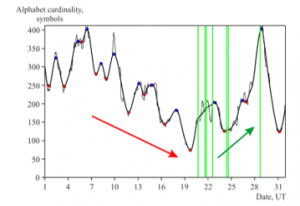
Figure 18: Graphs of AE signal alphabet cardinality dynamics in December 2018

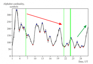
Figure 19: Graphs of AE signal alphabet cardinality dynamics in September 2019

The obtained estimates of the pre-seismic anomaly occurrence periods are consistent with the results of early studies. It was shown in [1, 2] that AE intensity increases at the frequency of 25 kHz 2–3 days before strong earthquakes. According to [16, 17], anomalies in the form of signal level increase appear in the frequency range of more than 6.5 kHz in the AE signals accumulated by 1 s. The results of time-frequency analysis of single AE pulses registered 1–7 days before earthquakes are presented in [18, 19]. According to these results, the number of pulses of a certain frequency increases before strong earthquakes. The above methods analyze signal frequency spectrum and, unlike the one described in the article, do not take into account waveform features. The proposed method of AE signals analysis updates the existing methodology and allows us to form more accurate short-term precursors of strong earthquakes.

Note that at all stages of the investigation, we had to face known nonlinear manifestations of the natural system under
the study. These manifestations reflected in the chaotic character of AE signal dynamic characteristics. As it had been expected,
the attempt of application of traditional methods for signal statistical processing, such as calculation of probability density function, ensemble averaging, estimation of statistic parameters
of different orders, to nonstationary AE signals did not provide stable results. Thus, the attention was focused on the search for invariant transformations which would be applied to AE chaotic character properly. On the whole, we think that we are
at the beginning of a perspective survey which, owing
to the chosen approach and the developed computer tools for analysis, will allow us to investigate deeper and to extend general and personal knowledge on seismic process behavior and, consequently, to predict catastrophic effects of earthquakes
at different stages and with more confidence.

6. Conclusions

A new method for analysis and classification of rock acoustic emission signals has been proposed. It is based on their symbol description. First of all, signal sections containing pulses
are determined. Each of the sections is described by a descriptive matrix. Based on the similarity degree of the descriptive matrices, pulses are structured into classes. Each class is considered
as a symbol and a set of obtained symbols composes an alphabet. Then we study the changes of alphabet parameters on signal subsequent fragments.

The developed method allows us to:

• distinguish informative features in AE signals based on their qualitative peculiarities;
• solve the problem of processing of a large volume of data by unifying pulse description and systematization;
• identify anomalies in AE signals distinguishing pre-seismic ones.

The method was implemented as an application program
by the means of which we analyzed acoustic emission signals which were recorded at “Karymshina” site of IKIR FEB RAS
in the seismically active region, Kamchatka peninsula, in 2016-2019. It was discovered during the analysis that in case of acoustic emission anomaly occurrence, alphabet content is redistributed
in favor of the symbols described by larger-size descriptive matrices (up to 350 extrema). Simultaneously with that the number of symbols increases. Analysis of alphabet averaged dynamics detected a clear tendency of alphabet cardinality decrease relatively the average 10–18 days before earthquakes and recovery of the value over the period from 2 to 8 days after them.

Thus, a new approach to the analysis of acoustic emission signals has been developed. The approach updates
the existing methodology of short-term earthquake precursor formation. On the basis of it, a system for automatic identification of pre-seismic AE anomalies can be created. It is topical for prediction of strong earthquakes which are catastrophic natural phenomena.

Conflict of Interest

The authors declare no conflict of interest.

Acknowledgment

The research was supported by the Russian Science Foundation, Project No. 18-11-00087.

1. G. Paparo, G. P. Gregori, U. Coppa, R. De Ritis, A. Taloni, “Acoustic Emission (AE) as a diagnostic tool in geophysics” Ann. Geophys-Italy, 45(2), 401–416, 2002. https://doi.org/10.4401/ag-3511
2. G. P. Gregori, G. Paparo, M. Poscolieri, A. Zanini, “Acoustic emission and released seismic energy” Nat. Hazard Earth Sys., 5, 777–782, 2005. https://doi.org/10.5194/nhess-5-777-2005
3. A. V. Kuptsov, “Variations in the geoacoustic emission pattern related to earthquakes on Kamchatka” Izv-Phys. Solid Eart+, 41(10), 825–831, 2005.
4. G. I. Dolgikh, V. A. Shvets, V. A. Chupin, S. V. Yakovenko, A. V. Kuptsov, I. A. Larionov, Y. V. Marapulets, B. M. Shevtsov, O. P. Shirokov, “Deformation and acoustic precursors of earthquakes” Dokl. Earth Sci., 413(1), 281–285, 2007. https://doi.org/10.1134/S1028334X07020341
5. G. P. Gregori, M. Poscolieri, G. Paparo, S. De Simone, C. Rafanelli, G. Ventrice, “Storms of crustal stress” and AE earthquake precursors” Nat. Hazard Earth Sys., 10, 319–337, 2010. https://doi.org/10.5194/nhess-10-319-2010
6. Y.V. Marapulets, B. M. Shevtsov, I. A. Larionov, M. A. Mishchenko, A. O. Shcherbina, A. A. Solodchuk, “Geoacoustic emission response to deformation processes activation during earthquake preparation” Russ. J. Pac. Geol., 6(6), 457–464, 2012. https://doi.org/10.1134/S1819714012060048
7. I. A. Larionov, Y. V. Marapulets, B. M. Shevtsov “Features of the Earth surface deformations in the Kamchatka peninsula and their relation to geoacoustic emission” Solid Earth, 5, 1293–1300, 2014. https://doi.org/10.5194/se-5-1293-2014
8. J. Serra, Image Analysis and Mathematical Morphology, Academic Press, 1982.
9. A. B. Tristanov, Yu. V. Marapulets, O. O. Lukovenkova, A. A. Kim, “A new approach to study of geoacoustic emission signals” Pattern Recognit. Image Anal., 26, 34–44, 2016. https://doi.org/10.1134/S1054661816010259
10. Yu. I. Senkevich, “The use of the empirical mode decomposition method to clean and restavration acoustic emission signal” E3S Web Conf., 62, 03008, 2018. https://doi.org/10.1051/e3sconf/20186203008
11. L. Alperovich, L. Eppelbaum, V. Zheludev, J. Dumoulin, F. Soldovieri, M. Proto, M. Bavusi, A. Loperte, “A new combined wavelet methodology applied to GPR and ERT data in the Montagnole experiment” J. Geophys. Eng., 10(2), 1–17, 2013. https://doi.org/10.1088/1742-2132/10/2/025017
12. O. Mandrikova, Yu. Polozov, N. Fetisova, T. Zalyaev, “Analysis of the dynamics of ionospheric parameters during periods of increased solar activity and magnetic storms” J. Atmos. Sol. Terr. Phy., 181, 116–126, 2018. https://doi.org/10.1016/j.jastp.2018.10.019.
13. O. Mandrikova, N. Fetisova, “Modeling and analysis of ionospheric parameters based on multicomponent mode” J. Atmos. Sol. Terr. Phy., 208, 105399, 2020. https://doi.org/10.1016/j.jastp.2020.105399
14. I. M. Johnstone, B. W. Silverman, “Needles and straw in haystacks: Empirical Bayes estimates of possibly sparse sequences” Ann. Statist., 32(4), 1594–1649, 2004. https://doi.org/10.1214/009053604000000030
15. I. M. Johnstone, B. W. Silverman, “Empirical Bayes selection of wavelet thresholds” Ann. Statist., 33(4), 1700–1752, 2005. https://doi.org/10.1214/009053605000000345
16. Y. Marapulets, O. Rulenko, “Joint Anomalies of High-Frequency Geoacoustic Emission and Atmospheric Electric Field by the Ground–Atmosphere Boundary in a Seismically Active Region (Kamchatka)” Atmosphere, 10(5), 267, 2019. https://doi.org/10.3390/atmos10050267
17. O. P. Rulenko, Yu. V. Marapulets, Yu. D. Kuz’min, A. A. Solodchuk, “Joint Perturbation in Geoacoustic Emission, Radon, Thoron, and Atmospheric Electric Field Based on Observations in Kamchatka” Izv-Phys. Solid Eart+, 55(5), 766–776, 2019. https://doi.org/10.1134/S1069351319050094
18. O. Lukovenkova, A. Solodchuk, “Analysis of geoacoustic emission and electromagnetic radiation signals accompanying earthquake with magnitude Mw = 7.5” E3S Web Conf., 196, 03001, 2020. https://doi.org/10.1051/e3sconf/202019603001
19. O. Lukovenkova, A. Solodchuk, A. Tristanov, E. Malkin, “Complex analysis of pre-seismic geoacoustic and electromagnetic emission signals” E3S Web Conf., 127, 03001, 2019. https://doi.org/10.1051/e3sconf/201912703001

(Click Here)

(Click Here)