1. Introduction

IoT is the combination of hardware environment, software services and Internet. It is composed of sensors, servers, hardware equipment, software equipment, and Internet connections [1]. With the fast improvement of sensors and devices, IoT could be applied to multiple fields such as wearables, smart home, and city. Face recognition is one of the popular personal security topics for IoT system, which could be widely used in personal home and public places security fields. Also, it has been used as an identification task in different areas, especially in corresponding with computer-based security and safety systems in homes, criminal identification, and smart phone devices’ face identification. For instance, cameras were used for image capturing and IoT processing devices, and Raspberry Pis, were used for comparing captured images with server database to provide directions over the GSM module and alert mobile phones [2]. Similar IoT systems with face recognition components were also proposed for security purposes in various applications, such as libraries and banks [3,4]. In this paper, we propose an effective segmented face recognition for IoT (SFR-IoT) shown in Figure 1.

Face recognition means recognize a specific person with a 2-D or 3-D face image or video base on available face data sets. If a camera is utilized to capture a suspect’s face image, that image can then be used to identify the suspect by using biometrics. The application of biometrics technology such as face recognition could reduce crime rates. Instead, the lack of effective skills in capturing biometric data from face images will potentially increase the opportunity for criminal activity [1].

Figure 1: Segmented Face Recognition Architecture (SFR-IoT)

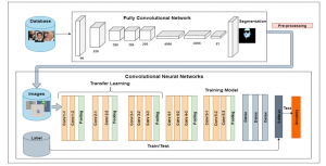
Figure 2: FCN-8Ss-VGG-16 System Architecture

Recently, a few researchers have published work related to crime detection. One study introduced a framework that first detects facial key points and then uses them to perform face recognition [2]. They mentioned that a larger number of images and camouflage images available in a data set can improve the training of the learning network and avoid the need to perform transfer learning. Results show that their framework outperforms the most advanced methods in critical point detection and facial camouflage classification.

For past investigation techniques, there are a few popular algorithms in regards to face cognition which include the geometric features method: principal component analysis (PCA) [3], linear discriminant analysis (LDA) [4], hidden Markov strategy (HMM) [5] and regular LBP features [6]. However, there are evident disadvantages in terms of utilizing these techniques. For instance, the accuracy rate of PCA will diminish significantly with lightness and a state of image change. Also, the strategy for inadequate data requires strict arrangement of information pictures, which is not applicable for basic application.

Due to the important factors of the accessibility of public data sets, as well as the improvement of Graphics Processing Unit (GPU) computation, neural networks has achieved a large renaissance, resulting in a significant increase in accuracy rates [7]. This leads to a major improvement in image recognition and finally in face recognition. For instance, Convolutional Neural Network (CNN) [8,9] is a popular model in neural networks. It is a state-of-the-art technique that has replaced the traditional algorithms on face recognition and consequently taken the network by storm, fundamentally enhancing the cutting edge in numerous applications. Several studies have applied CNN for face recognition purposes, such as Deep Face [10], DeepID3 [11] and Face Net [12]. They have achieved around 97%, 99.6%, and 99.5% success rates, respectively.

     Recent studies that combined face segmentation and face recognition technology have provided an important concept for our research. For example, one study extracted face-like regions by using the extracted color information of an image in HSV color space, and the RHT algorithm is then applied to find face region [13]. Samantha proposed a technology of segmentation skin color through YcbCr as well, then applied artificial neural network classified face and non-face classes [14]. However, these researches did not integrate deep learning study for face segmentation and recognition, so this paper would like to propose a new methodology that improve the deficiency.

Even though current automated face recognition systems can recognize individual faces in controlled environments with a 99% accuracy, the accuracy drops to below 60% when images are in unconstrained environments [15].

This is caused by rich facial expressions and changing gestures; face movements with lights; angle; and distance [2].

In addition, disguised faces with glasses, scarves, and accessories will become challenging elements in face recognition tasks. Hence, in order to explore a more effective method to solve this problem, this study proposes a new system called FCN-8s-VGG-16, which is used for the segmentation technology face recognition before classification. The system contains two procedures, as shown in Figure 2. The process of this research is to build a training set of segmentation of the face area with FCN as an input of Convolution Neural Network (CNN), and then train the CNN network from VGG-Face with transfer learning. Lastly, the classification function SoftMax is applied for face probability distribution. The first step is to  segment the original image for extracting face parts (eyes, nose, mouth, and skin) from the background, which applies a pre-trained FCN-8s model [16]. Secondly, the output images are fed into the network applying transfer learning [10] based on VGG-16 [8] with our fine-tuned technology on face recognition task. Finally, the Softmax function calculates the probability distribution of the test image and generates the accuracy rate while comparing it to the label box.

2. Related Work

2.1.  General Segmentation and Face Segmentation

Segmentation refers to the process of separating an image or frame into groups of pixels which are identical with respect to some standard. A few papers have applied segmentation for their research topic.

In [17], the author proposed a food calorie estimation model, which was applied on a smartphone to predicate calories of the food in images taken by a phone camera. Firstly, they estimated approximate positions of dishes by edge detection. Secondly, k-means based clustering was applied on the color pixels, thereby extracting a bounding box of a food area. Next, they used GrabCut [18] to obtain an accurate food area within the estimated bounding box. Then, they employed CNN as a calorie estimation task. They prepared 120-calorie annotated food photos as the data for the experiments. Finally, 60 test images with real food calories are estimated with the relative average error of 21.3%, regarding food calorie prediction achieved, and it is higher than the Japanese government definition.

In [19], the author applied different segmentation techniques in the aim of reorganization of the left ventricle in a VEF image. He compared two segmentation approaches: region-based segmentation and edge-based segmentation. The first detects homogeneities and the common features by simultaneously applying the chan_vese model and the thresholding techniques. In the second approach, he applied a certain algorithm such as Sobel, Canny, and Perwitt to obtain the interim between two related regions. Results showed that region-based segmentation using the chan_vese model in conjunction with thresholding gives a better performance.

Since Convolution Neural Network (CNN) has been widely researched by the scholarly field, various models and systems with different purposes are dramatically increased. Fully Convolution Network (FCN) [20] is one of most popular image segmentation technology that is widely used in studies. FCN extracts pixels from CNN layers of mixed scales, enlarges them to the size of the original image, and then applies a convolution layer to classify all this information.

There are research works pertaining to FCN for segmentation purposes that have achieved excellent results. One study presented a One-Shot Video Object Segmentation (OSVOS) based on the FCN network architecture, with transfer learned on ImageNet then fine-tuned on one training sample [21]. The performance was tested on DAVIS database, which consists of 50 full-HD video sequences and YouTube objects. The result shows that OSVOS is fast and improves the state-of-the-art technology by a significant margin (79.8% vs 68.0%). Based on these outstanding results, this paper chooses FCN as our face extraction segmentation tool.

In [22], the author proposed a method to achieve the segmentation of skin, hair, and background by applying FCN-8s and fully-connected CRF. Next, matting algorithm was facilitated in their experiment in order to receive clear hair and skin alpha masks. Finally, they demonstrated that state-of-the-art performance on LFW Parts dataset [23] holds more accurately than other approaches. The defect of the FCN algorithm influences our decision to apply Transfer Learning in our experiment, which we will talk about it in Chapter 3.

2.2.  Face Recognition

Another study has shown that choosing an appropriate model in CNN architecture is vital for face recognition. This study evaluated two popular CNN architectures, Alex-Net [9] and VGG-16 [8], on face recognition. They accomplished their task by transferring learning idea to the networks trained for various classifying purposes. One study [24] used Alex-Net model to train the CASIA-WebFace [25] database, and the research shows that VGG performs better than Alex-Net. This paper inspired us to employ VGG-16 [8] as a face recognition model for our own experiment.

In [26], the author conducted face recognition by applying a CNN for feature extraction. First, they randomly selected patches from the STL-10 [27] database and used them to train a linear decoder and obtain a 400 × 192 learned weights matrix. The 64 × 64 RGB images are used to train the identifier through a convolutional layer, and then training features are extracted using these learned weights. Results show the proposed method reached a high rate of excellent sorting, ranging from about 80% to 100%.

There is another study [28] that has proposed a modified Convolutional Neural Network (CNN) architecture with the addition of two batch normalization operations on two of the layers. CNN architecture was utilized to separate particular face features, and Softmax classifier was utilized to recognize faces in the completely associated layer of CNN. The training and test process were tested on a Georgia Tech face database. After pre-processing, the researchers changed the sizes of input to 16×16×1, 16×16×3, 32×32×1, 32×32×3, 64×64×1, and 64×64×3 in order to receive the best result. Finally, 64x64x3 surpasses other sized images regarding the lowest Top-1 error rate. Our paper applied a similar strategy with this research, through altering the size of input in order to obtain the best result in our experiment.

However, to our knowledge, segmentation technology is not used in the face recognition field so far, except in our initial work [29]. This paper is an extension of work originally presented in the 2019 18th IEEE International Conference on Machine Learning and Applications. The accuracy rate will increase due to the interference decrease from unrelated face pixels, such as glasses. In order to decrease the useless effect pixels of disguised face parts, this study would like to propose an FCN-8s-VGG-16 system with segmented technology before classification. It only keeps face sections, and the other parts will be taken off. For the purpose of examination both before and after the change, the face section is sent to the classification model and accuracy will be tested for comparison.

3. The Proposed Approach

3.1. Methodology (CNN)

3.1.1. VGG-16

The core idea of convolutional networks is classifying target data samples to the different distances between classes. The network structure includes three convolutions (conv1, conv2, conv3), two pooling layers (Pool1, Pool2), and a fully connected layer [8].

3.1.2.         Convolution Layer

The input data is trained by employing a set of trainable neurons. The output of each of the feature maps corresponds to an image filter of the same size as the input of the convolution layer. The primary function of the convolution layer is to extract features from an image. Every convolution layer is trained on a feature map of the past layer, sequentially, and then it usually adds a bias parameter in order to increase accuracy by activating the function to translate results from linear to non-linear function. After that, the feature maps are fed into the next convolutional layer as input data.

3.1.3.         Pooling Layer

Pooling layer decreases the dimensionality of each activation map but keeps the most vital data information. The input images are separated into a set of non-covering square shapes. Each field is downsampled by a non-linear function. For example, average or maximum is used the most. This layer accomplishes a better speculation and robust result for system.

3.1.4.         ReLU Layer

Rectified linear units (ReLU) is a non-linear operation. It is an important function because it ends up with 0 if the input is less than 0. However, if the input is greater than 0, the output will be an original number. Research studies show that ReLU results can implement faster training for a huge network.

3.1.5.         Fully Connected Layer

The output from convolution layer, pooling layer, and ReLU layer is high- level features of input data. The purpose of applying the Fully Connected Layer (FCL) is to sum these features for classifying the input data into different classes based on the probability of each class of each feature map. Next, FCL supports the features to a classifier, which is Softmax function. This function will conclude the probabilities of every target class over all possible target instances. Afterwards, the calculated probabilities will decide the target class for the given inputs.

3.1.6.         Why VGG

There are a few CNN architectures, such as LeNet, AlexNet, Reset, and so on, which have been widely used since CNN was invented. Recently, the most state-of-the-art model [10] outperforms in the localization and recognition tracks, respectively, the ImageNet Challenge 2014 among them.

This VGG model is described by its simplicity, applying only 3×3 filters stacked over each other in increasing depth. Reducing parameter numbers and model size is employed by max pooling, two fully-connected layers, each with 4,096 nodes followed by a Softmax classifier.

3.1.7.         Transfer Learning

Transfer learning is an area of artificial intelligence, which centers around the capacity for a machine learning calculation to enhance learning limits on a target data set through past exposure to an alternate way. The measured quality of a CNN implies that we can easily apply the weights from a pre-trained model and only re-prepare most elevated layers. In particular, we re-prepare all linear layers in the model and replace parameters of the highest layers in VGG-16 [8]. To get rid of the lack of geometric invariance of these approaches, fine-tuning [30] with an external data set can be utilized. The primary distinction between picture arrangement and picture recovery is the measure of information and its fluctuation. In classification, it is important to use huge data sets with high variability for different categories. However, in image recognition, the geometric invariance of an image is less essential for a training model. As the purpose of image recognition is to recognize the instance of example, less variability data will be needed.

In this paper, to use CNN functionally, we fine-tune the pre-trained CNN [10] a face data set for image recognition. Fine- tuning usually focuses on the higher layers while fixing the lower layers of a CNN. We use FCN-8s-VGG [16] architecture, which has been pre-fine-tuned for segmentation on PASCAL [31]. As the CNN model [16] is pre-trained on face dataset and performs an excellent result, we don’t consider it for Fine-tuning while we are doing the same object segmentation purpose.

Table 1: The Architecture of VGG-Face Refined

Layer	Layer Type	Filters	Input	Training
1	Conv.	64	3x3x3	False
2	Conv.	64	3x3x64	False
3	Max-Pool	–	2×2	–
4	Conv.	128	3x3x64	False
5	Conv.	128	3x3x128	False
6	Max-Pool	–	2×2	–
7	Conv.	256	3x3x128	False
8	Conv.	256	3x3x256	False
9	Conv.	256	3x3x256	False
10	Max-Pool	–	2×2	–
11	Conv.	512	3x3x256	True
12	Conv.	512	3x3x512	True
13	Conv.	512	3x3x512	True
14	Max-Pool	–	–	–
15	Conv.	512	3x3x512	True
16	Conv.	512	3x3x512	True
17	Conv.	512	3x3x512	True
18	Max-Pool	–	2×2	–
19	FC	–	4096	True
20	FC	–	4096	True
21	FC	–	85	True
22	Softmax	–	–	–

3.1.8.  VGG-FACE

VGG-Face [10] is a model that was pre-trained based on the VGG-16 structure and set up on a face data set acquired by the Visual Geometry Group that is comprised of more than 2.5 million pictures and 2,622 different labels. Detailed information in terms of VGG-16 model was shown in Table 1, including layer types, number of filters, and input image size.

The architecture of VGG-face contains a total of 22 layers: 13 convolutional layers for image and filter calculation, 5 max pooling layers for keeping feature information, 3 fully connected layers for summing up all previous features, and later a Softmax layer for classification [10]. The normal image resolution of the input layer is 224×224. Table 1 shows the detailed architecture of the VGG-face, including filter numbers and input size at each layer applied in our research. In this experiment, we have fixed the previous 10 layers and changed 21 fully connected layers from 1,000 to 85, since we have 85 classes in the experiment, which means 85 labels will be generated. Additionally, we fixed the parameters of the lower convolutional layers from 1-9 but trained the higher convolutional layers from 11-17 and the FCN layers from 19-21. Applied changes are highlighted in the table.

3.2.  Methodology (FCN)

FCN [16] uses the identical convolutional network based on VGG-16 layers [8] and converts the fully connected layer to a convolutional layer. In the traditional CNN structure, the first five layers are convolutional layers, and the sixth and seventh layers are a one-dimensional vector with a length of 4096. The eighth layer is a one-dimensional vector with a length of 1,000, corresponding to 1,000 different probabilities of the category. Instead, FCN represents these three layers as a convolutional layer whose size (number of channels, width, height) is (4096, 1, 1), (4096, 1, 1), (1000, 1, 1), respectively. There does not seem to be any difference in numbers, but convolution is not the same concept, and calculation process as a fully-connected layer. The convolutional layer uses the weights and biases that CNN has pre-trained, but the difference is that the weights and offsets are their own scope and belong to their own convolution kernel. Therefore, all layers in the FCN network are convolutional layers and are called fully convolutional networks.

3.2.1. Upsampling

Upsampling is also called deconvolution at some points, as both of their operations are multiplication and addition. The upsampling of the accompanying factor f is a convolution operation on a fractional input with a step size of 1/f.

Backward convolution is called deconvolution. Meanwhile, the forward and backward propagation of upsampling can only be achieved by reversing the forward and backward propagation of the convolution. Consequently, it performs well no matter the optimization or backward propagation. Deconvolution can enlarge input size by learning parameters while training [20].

3.2.2. Skip Layers

Now that we have a 1/32 size, a 1/16 size, and a 1/8 size feature map, after upsampling the 1/32 size heatmap, the image restored by this operation is a convolutional kernel of conv5. The features are limited to the accuracy, so they cannot restore the features in the image well; consequently, forward propagation will be applied. Detailed information could be complemented by upsampling the conv4. Afterwards, conv3 does the exact same calculation as conv4. Finally, the process completes the restoration of the entire image. According to different strides with 32, 16, and 8, FCN splits into three kinds of results: FAC-32s, FCN-16, and FCN-8s [20]. Obviously, FCN-8s combined previous FCN-32s and FCN-16 results, which gives FCN-8s more accuracy. We decided to choose FCN-8s in our experiment.

3.2.3. Why choosing FCN

The reason why this research employs FCN are below:

• Traditional segmentation method segmented the image into similar sections, including coherent area-independent, low-level clues based on categories, such as pixel color or proximity. Semantic segmentation, on the other hand, assigned each pixel of the image to a semantic tag. This usually means classifying each pixel (for example: the pixel 1 belongs to the glass, the pixel 2 belongs to the hair). Pixel-level classification seems more efficient than cutting out each patch [32]. The FCN-8s model brings state-of-the-art performance on PASCAL VOC in 2011 and 2012 [20].
• No fully connected layer is used in this kind of architecture, which reduces the number of parameters and the computation time. In addition, the network works regardless of the original image size. It could be trained from small and big images, and it does not require any particular number of units at any stage. Additionally, all connections are local [20]. FCN brought great breakthroughs on semantic segmentation tasks when implemented on image segmentation [20].

It is tough to obtain millions of diverse images with ground truth segmentation labels, which could be difficult and mostly performed manually. However, it is convenient to use a pre-trained model for research purposes. Our method applies the FCN segment to the visible parts of faces from their specific circumstance and impediments, which is a fine-tuned system for face segmentation on PASCAL [20] on the data set of IARPA Janus CS2 [33] with 9,818 segmented faces achieved.

Figure 3:  FCN-8s-VGG-16 System 2

This research has achieved an excellent segmentation performance that could be obtained with a standard FCN trained on plenty of rich and varied examples. FCN-8s combined previous FCN-32s and FCN-16s results, which gives FCN-8s more accuracy. We decided to choose FCN-8s in our experiment. Figure 3 shows the process of our experiment.

3.3.  Methodology

3.3.1. Data selection

The ImageNet Large Scale Visual Recognition Challenge (ILSVRC) [34] was dominant in giving this information to the general picture classification task. Moreover, analysts have made data sets accessible for object recognition [35]. Labeled Faces in the Wild (LFW) [36],  as the most popular benchmark data set has dominated in the field of face recognition for many years. It is a

Figure 4:  Gallery Images

huge scale open data set and the benchmark database of face photos intended for concentrating the issue of unconstrained face recognition, which has been widely applied in numerous research studies [10,12]. The data set contains more than 13,000 images of face pictures gathered from online.

Each face has been labeled according to the name of the individual envisioned. However, due to the shortage of obvious challenging face images, such as block face, tilt the head, wrinkle the eyebrows, and so on, it is not an ideal image set in terms of the purpose of the paper, which is to compare face recognition performance with and without segmentation. Furthermore, FRGC [37] MS-celeb-1M [38] and MOBIO [39] are other benchmark face data sets used to identify face images though various experiments with the same problem as LFW.

3.3.2. Applied Data Set

In this research, we decided to employ the Celebrity-Face-Recognition-Dataset, which consists of 1,100 famous  celebrities with 8,000 images [40] in each. In this dataset, the total size of the data set is 172 GB with 800*800*3 pixels in each. Due to the limitations of our hard drive and memory, this research randomly and manually selected 85 individuals with 100 images for each as classes for the face recognition task.

Since accuracy difference along with and without segmentation face section from the background is in a significant index for the research, the images with obvious covers such as hats, accessories, or different poses and hairstyles, are our preferred selection among the 8,500 figures from the Celebrity-Face-Recognition dataset. Figure 4 shows partial data processed in our experiment.

3.3.3. Data Augmentation

Image recognition technology focuses on the work of few data sets and small variability in object images. This results in very few images that can train a particular CNN model, even with fine-tuning. One way to solve this problem is to augment the data, by randomly applying transformations, color perturbations, and other random transformations. Randomly rotating and flipping the images can make up the deficiency of diversity pixels of the model. In the experiment, the following values are applied:

• Brightness: Images are randomly changing brightness [-0.1, 0.1) [41].
• Flipping: Images are horizontally flipped from left to right.
• Scaling: The pixel values are scaled to the range [0, 1].
• Contrast: Images are randomly adding contrast to the range [0.2, 1.8].

The result shows below as Figure 5.

Figure 5:  Pre-processing Result with FCN-8s Segmentation

3.3.4. Cross Validation

 We found that in using the same data set, both training and model error estimation, the error estimation is mostly inaccurate, which is called the optimism of the model error estimation. To overcome this problem, cross-validation was proposed. According to Kohavi [42], cross-validation is a technology used to access predictive systems by dividing the original data set into a training set for training the parameters, with a test set for assessing the trained model. There are three more popular methods: leave-one-out, leave-P-out, and K-fold. Compared to the previous two technologies, K-fold only needs to calculate k times, which dramatically decreases code complexity. In K-fold cross-validation, the input data is split into k same size subsets, which is called folds as well. K-1 subset data will be trained into a system afterward, assessing the model on the subset that was not utilized for preparing. This procedure is repeated k times (the folds) until each subset has been used for evaluation purposes (and prohibited from training) each time finished. The results from k times calculation of K-folds can then be averaged (or joined) to receive a final estimation. The advantage of this method is that all data information is used for both training and evaluation, and each sub-dataset is used for validation exactly once. Based on the advantage of cross-validation, this paper has applied the 10-folds cross- validation on a data set.

3.3.5.  Hardware Utility

Our implementation is based on Tensorflow Framework. AWS as a service platform that support the measurement of runtimes and performance. We implemented the experiment on the 16 GB memory of Nvidia Tesla 100V GPU.

4. Experimental Results

During this examination process, the implementation of the proposed method has been evaluated based on the percentage recognition rate of the identities on the testing data set. Initially, we set the learning rate as 0.001 for the CNN system, and a total of 10,000 steps are required for every k times calculation. Then for each step, 10 images (batch size) and 20 images (batch size) are sent for training through the network individually. At the same time, a 50% dropout was also been used in the experiment. Rectified Linear Unit (ReLU) as activation functions and Cross Entropy Loss function are applied to guide CNN training. The Adam algorithm calculates the gradient of entire data sets and updates values in the opposite direction to the gradients until a local minimum is found. Top-1 accuracy is applied to measure the performance of processes. This entire test experiment will be repeated ten times until the average of performance is obtained. The results of our experiment are used to compare with the performance of others. To check and analyze the implementation of the proposed method, 10 image samples from each category are collected into the test set.

According to the outstanding performance of our experiment, we took the best parameter as the final performance and compared it with the model consisting of original images. We performed various experiments by altering the image size. For example, we drafted the size of each picture after pre-processing as 350x350x3, 500x500x3, and 800x800x3. Among the data set, 90% of the data are the training set and 10% are the test set. 10,000 steps were applied for CNN training process ten times.  Based on Top-1 error calculation, the result of the proposed system was acquired. According to whether the prediction is the same as the target category, the Top-1 error rate returns a Boolean value.

Table 2: Performance Comparison with Various Parameters

Input Image size	Numbers steps	Learning rate	Batch size	(VGG-16 System) Top1      Error	(Proposed    FCN-8s-VGG-16 system) Top1 Error
350x350x3	10000	0.001	10	82.69%	92.15%
350x350x3	10000	0.001	20	84.34%	93.21%
500x500x3	10000	0.001	10	92.43%	97.25%
500x500x3	10000	0.001	20	93.54%	98.33%
800x800x3	10000	0.001	10	99.84%	99.57%
800x800x3	10000	0.001	20	99.88%	99.69%

     Table 2 shows the comparison performance of various parameters. As seen from Table 2, the input size of 350x350x3 and 500x500x3 of the FCN-8s-VGG-16 system obtained a higher accuracy rate than the VGG-16 System which is trained without segmentation technology. Meanwhile, the accuracy rate of 800x800x3 input size achieved the closest result with the VGG-16 System. Furthermore, the running time has reduced on average 4.52% than the VGG-16 System in all three experiments owing to reduced pixel with segmentation technology. Figure 6 demonstrates the relationship between the batch size, image size and the system. We can conclude that as the batch size increased, both accuracy rate of VGG-16 System and FCN-8s-VGG-16 have increased slightly.

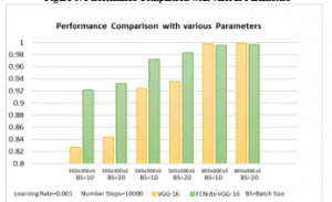
Figure 6: Performance Comparison with various Parameters

However, this will expand running time as well. Therefore, the batch size and running time could be a future trade off work for us.  Above all, we could gather that image input size with high pixels will have a higher accuracy rate for recognition.

5. Conclusion and Future Work

In this paper, we proposed the FCN-8s-VGG-16 system to segment face images and recognize segmented images with high precision. Our face recognition system, FCN-8s-VGG-16 is composed of face image segmentation with FCN-8s [16] and  VGG-Face fine-tuning model recognition. Experiments were conducted on Celebrity-Face-Recognition dataset [40] for training and testing purposes. Compared with the original face recognition without segmentation accuracy, the effective classification rate using different parameters has been significantly improved from 92.15% to 99.69%, reaching a level of 82.69% to 99.88%. It also demonstrates that increasing the size of the input and batch number, while keeping the learning rate and number of steps constant, will improve the accuracy rate in certain situations. However, such observation is not completely ensured for other systems.

Accuracies on Top-1 in face recognition results means that some limitations happened in our algorithm, especially when applied to a wild data sets: First, even though FCN-8s has successfully segmented most face images, there were still a few images that did not achieve ideal results. For example, some small black areas occur after segmentation, which will affect the accuracy of performance. There are a few things that have triggered these failures. First, it takes three training processes to get the FCN-8s, which is not sensitive enough to combine the details of the image. This is because when the decoding is performed, that is, when the original image is restored, the label map of the input upsampling layer is too sparse. Secondly, FCN-8s does not consider the relationship between pixels during classification, and it lacks spatial consistency. Additionally, we only computed limited image input size, batch sizes, and learning rate, so it is very possible that we will receive a better accuracy rate if there are more parameters to choose from, with time allowed. Lastly, with the fine-tuning FCN model [16], the model will be more robust [43]. Only one recognition model processed in the experiment is limited. Some other CNN model has achieved an excellent performance in recent competition. For example, Google Net [44] is a winning architecture on ImageNet 2014. We will be applying it as our recognition system in future research for comparing with VGG-16. Besides, in reality, a human face is made of a 3D model; it’s more realistic to segment and recognize images based on 3D faces. [45] has proposed a system of face recognition 3D based on segmentation by classifying fields of facial images before and after fusion of color and depth images. It brings us a potential research in face recognition study that we could investigate more about 3D image segmentation technologies instead of 2D.

Additionally, we will develop a mobile app such as [5], to complete the SFR-IoT architecture that could receive notification from our system though IoT devices when recognizing face in order to make contribution in real world application. In the future, data encoding and decoding will be applied to untrusted devices and servers to protect privacy data to make software more powerful and trustworthy [46].

Above all, the comparison reveals significant improvement in performance. Further experiments can be done by improving segmentation technology or by changing the recognition model.

1. S. Zalke, P.M.-2015 I.C. On, U. 2015, Survey on implementation of enhanced uniform circular local binary pattern algorithm for sketch recognition, Oct. 2020.
2. J. Cui, J. Li, Y.H.-2008 I.C. on, undefined 2008, “Research on Face Recognition Method based on Cognitive Mechanism,” Ieeexplore.Ieee.Org, Oct. 2020.
3. X. Dong, H. Huang, H.W.- ISCSCT, undefined 2010, “A comparative study of several face recognition algorithms based on pca.”
4. H. Yu, J. Yang, “A direct LDA algorithm for high-dimensional data — with application to face recognition,” Pattern Recognition, 34(10), 2067–2070, 2001, doi:10.1016/s0031-3203(00)00162-x.
5. J. Bobulski, “Face recognition method with two-dimensional HMM,” in Advances in Intelligent Systems and Computing, Springer Verlag: 317–325, 2016, doi:10.1007/978-3-319-26227-7_30.
6. T. Ojala, M. Pietikäinen, D. Harwood, “A comparative study of texture measures with classification based on feature distributions,” Pattern Recognition, 29(1), 51–59, 1996, doi:10.1016/0031-3203(95)00067-4.
7. S. Zalke, P.S. Mohod, “Survey on implementation of enhanced uniform circular local binary pattern algorithm for sketch recognition,” in ICIIECS 2015 – 2015 IEEE International Conference on Innovations in Information, Embedded and Communication Systems, Institute of Electrical and Electronics Engineers Inc., 2015, doi:10.1109/ICIIECS.2015.7192917.
8. S. Karen, Z. Andrew, “VERY DEEP CONVOLUTIONAL NETWORKS FOR LARGE-SCALE IMAGE RECOGNITION Karen,” American Journal of Health-System Pharmacy, 75(6), 398–406, 2018.
9. A. Krizhevsky, I. Sutskever, G.E. Hinton, “ImageNet classification with deep convolutional neural networks,” Communications of the ACM, 60(6), 84–90, 2017, doi:10.1145/3065386.
10. O.M. Parkhi, A. Vedaldi, A. Zisserman, “Deep Face Recognition,” in Procedings of the British Machine Vision Conference 2015, British Machine Vision Association: 41.1-41.12, 2015, doi:10.5244/C.29.41.
11. D. Virmani, T. Sharma, M. Garg, GAPER: Gender, Age, Pose and Emotion Recognition Using Deep Neural Networks, Springer, Singapore: 287–297, 2021, doi:10.1007/978-981-15-5463-6_26.
12. F. Schroff, D. Kalenichenko, J. Philbin, “FaceNet: A unified embedding for face recognition and clustering,” Proceedings of the IEEE Computer Society Conference on Computer Vision and Pattern Recognition, 07-12-June, 815–823, 2015, doi:10.1109/CVPR.2015.7298682.
13. A. Aminian, M.S. Beni, “Face detection using color segmentation and RHT,” in 3rd International Conference on Pattern Analysis and Image Analysis, IPRIA 2017, Institute of Electrical and Electronics Engineers Inc.: 128–132, 2017, doi:10.1109/PRIA.2017.7983032.
14. S.D.F. Hilado, E.P. Dadios, R.C. Gustilo, “Face detection using neural networks with skin segmentation,” in Proceedings of the 2011 IEEE 5th International Conference on Cybernetics and Intelligent Systems, CIS 2011, 261–265, 2011, doi:10.1109/ICCIS.2011.6070338.
15. J.C. Klontz, A.K. Jain, “A case study of automated face recognition: The Boston marathon bombings suspects,” Computer, 46(11), 91–94, 2013, doi:10.1109/MC.2013.377.
16. Y. Nirkin, I. Masi, A.T. Tuǎn, T. Hassner, G. Medioni, “On face segmentation, face swapping, and face perception,” in Proceedings – 13th IEEE International Conference on Automatic Face and Gesture Recognition, FG 2018, Institute of Electrical and Electronics Engineers Inc.: 98–105, 2018, doi:10.1109/FG.2018.00024.
17. K. Okamoto, K. Yanai, “An automatic calorie estimation system of food images on a smartphone,” in MADiMa 2016 – Proceedings of the 2nd International Workshop on Multimedia Assisted Dietary Management, co-located with ACM Multimedia 2016, Association for Computing Machinery, Inc: 63–70, 2016, doi:10.1145/2986035.2986040.
18. C. Rother, V. Kolmogorov, A. Blake, “‘GrabCut’ – Interactive foreground extraction using iterated graph cuts,” in ACM Transactions on Graphics, 309–314, 2004, doi:10.1145/1015706.1015720.
19. Y. Ben Fadhel, S. Ktata, T. Kraiem, “Cardiac scintigraphic images segmentation techniques,” in 2nd International Conference on Advanced Technologies for Signal and Image Processing, ATSIP 2016, Institute of Electrical and Electronics Engineers Inc.: 364–369, 2016, doi:10.1109/ATSIP.2016.7523107.
20. J. Long, E. Shelhamer, T. Darrell, “Fully convolutional networks for semantic segmentation,” in Proceedings of the IEEE Computer Society Conference on Computer Vision and Pattern Recognition, IEEE Computer Society: 431–440, 2015, doi:10.1109/CVPR.2015.7298965.
21. S. Caelles, K.-K. Maninis, J. Pont-Tuset, L. Leal-Taixé, D. Cremers, L. Van Gool, “One-Shot Video Object Segmentation,” Proceedings – 30th IEEE Conference on Computer Vision and Pattern Recognition, CVPR 2017, 2017-January, 5320–5329, 2016.
22. S. Qin, S. Kim, R. Manduchi, “Automatic skin and hair masking using fully convolutional networks,” in Proceedings – IEEE International Conference on Multimedia and Expo, IEEE Computer Society: 103–108, 2017, doi:10.1109/ICME.2017.8019339.
23. LFW Face Database | Part Labels, Oct. 2020.
24. D. Bussey, A. Glandon, L. Vidyaratne, M. Alam, K.M. Iftekharuddin, “Convolutional neural network transfer learning for robust face recognition in NAO humanoid robot,” in 2017 IEEE Symposium Series on Computational Intelligence, SSCI 2017 – Proceedings, Institute of Electrical and Electronics Engineers Inc.: 1–7, 2018, doi:10.1109/SSCI.2017.8285347.
25. D. Yi, Z. Lei, S. Liao, S.Z. Li, “Learning Face Representation from Scratch,” 2014.
26. A. Raj, S. Gupta, N.K. Verma, “Face detection and recognition based on skin segmentation and CNN,” in 11th International Conference on Industrial and Information Systems, ICIIS 2016 – Conference Proceedings, Institute of Electrical and Electronics Engineers Inc.: 54–59, 2016, doi:10.1109/ICIINFS.2016.8262907.
27. STL-10 dataset, Oct. 2020.
28. M. Coskun, A. Ucar, O. Yildirim, Y. Demir, “Face recognition based on convolutional neural network,” in Proceedings of the International Conference on Modern Electrical and Energy Systems, MEES 2017, Institute of Electrical and Electronics Engineers Inc.: 376–379, 2017, doi:10.1109/MEES.2017.8248937.
29. F. Gao, J. Liu, “Face recognition using segmentation technology,” in Proceedings – 18th IEEE International Conference on Machine Learning and Applications, ICMLA 2019, Institute of Electrical and Electronics Engineers Inc.: 545–548, 2019, doi:10.1109/ICMLA.2019.00102.
30. A. Babenko, A. Slesarev, A. Chigorin, V. Lempitsky, “Neural Codes for Image Retrieval,” Lecture Notes in Computer Science (Including Subseries Lecture Notes in Artificial Intelligence and Lecture Notes in Bioinformatics), 8689 LNCS(PART 1), 584–599, 2014.
31. The PASCAL Visual Object Classes Homepage, Oct. 2020.
32. G. Csurka, D. Larlus, F. Perronnin, “What is a good evaluation measure for semantic segmentation?,” BMVC 2013 – Electronic Proceedings of the British Machine Vision Conference 2013, 2013, doi:10.5244/C.27.32.
33. B.F. Klare, B. Klein, E. Taborsky, A. Blanton, J. Cheney, K. Allen, P. Grother, A. Mah, M. Burge, A.K. Jain, “Pushing the frontiers of unconstrained face detection and recognition: IARPA Janus Benchmark A,” Proceedings of the IEEE Computer Society Conference on Computer Vision and Pattern Recognition, 07-12-June, 1931–1939, 2015, doi:10.1109/CVPR.2015.7298803.
34. O. Russakovsky, J. Deng, H. Su, J. Krause, S. Satheesh, S. Ma, Z. Huang, A. Karpathy, A. Khosla, M. Bernstein, A.C. Berg, L. Fei-Fei, “ImageNet Large Scale Visual Recognition Challenge,” International Journal of Computer Vision, 115(3), 211–252, 2014.
35. T.Y. Lin, M. Maire, S. Belongie, J. Hays, P. Perona, D. Ramanan, P. Dollár, C.L. Zitnick, “Microsoft COCO: Common objects in context,” in Lecture Notes in Computer Science (including subseries Lecture Notes in Artificial Intelligence and Lecture Notes in Bioinformatics), Springer Verlag: 740–755, 2014, doi:10.1007/978-3-319-10602-1_48.
36. G.B. Huang, M. Ramesh, T. Berg, E. Learned-Miller, Labeled Faces in the Wild: A Database for Studying Face Recognition in Unconstrained Environments, Oct. 2020.
37. P.J. Phillips, P.J. Flynn, T. Scruggs, K.W. Bowyer, J. Chang, K. Hoffman, J. Marques, J. Min, W. Worek, Overview of the Face Recognition Grand Challenge *, 2005.
38. Y. Guo, L. Zhang, Y. Hu, X. He, J. Gao, “MS-Celeb-1M: A Dataset and Benchmark for Large-Scale Face Recognition,” 2016.
39. C. McCool, S. Marcel, A. Hadid, M. Pietikäinen, P. Matějka, J. Černocký, N. Poh, J. Kittler, A. Larcher, C. Lévy, D. Matrouf, J.F. Bonastre, P. Tresadern, T. Cootes, “Bi-modal person recognition on a mobile phone: Using mobile phone data,” in Proceedings of the 2012 IEEE International Conference on Multimedia and Expo Workshops, ICMEW 2012, 635–640, 2012, doi:10.1109/ICMEW.2012.116.
40. GitHub – prateekmehta59/Celebrity-Face-Recognition-Dataset: Dataset of around 800k images consisting of 1100 Famous Celebrities and an Unknown class to classify unknown faces, Oct. 2020.
41. J.J. Lv, X.H. Shao, J.S. Huang, X.D. Zhou, X. Zhou, “Data augmentation for face recognition,” Neurocomputing, 230, 184–196, 2017, doi:10.1016/j.neucom.2016.12.025.
42. R. Kohavi, A Study of Cross-Validation and Bootstrap for Accuracy Estimation and Model Selection, 1995.
43. Y. Sun, D. Liang, X. Wang, X. Tang, “DeepID3: Face Recognition with Very Deep Neural Networks,” 2015.
44. C. Szegedy, W. Liu, Y. Jia, P. Sermanet, S. Reed, D. Anguelov, D. Erhan, V. Vanhoucke, A. Rabinovich, “Going deeper with convolutions,” in Proceedings of the IEEE Computer Society Conference on Computer Vision and Pattern Recognition, IEEE Computer Society: 1–9, 2015, doi:10.1109/CVPR.2015.7298594.
45. M. Belahcene, A. Chouchane, M. Amin Benatia, M. Halitim, “3D and 2D face recognition based on image segmentation,” in 2014 International Workshop on Computational Intelligence for Multimedia Understanding, IWCIM 2014, Institute of Electrical and Electronics Engineers Inc., 2014, doi:10.1109/IWCIM.2014.7008800.
46. W. Xue, W. Hu, P. Gauranvaram, A. Seneviratne, S. Jha, “An Efficient Privacy-preserving IoT System for Face Recognition,” in Proceedings – 2020 Workshop on Emerging Technologies for Security in IoT, ETSecIoT 2020, Institute of Electrical and Electronics Engineers Inc.: 7–11, 2020, doi:10.1109/ETSecIoT50046.2020.00006.

(Click Here)

(Click Here)