1. Introduction

This paper is an extension of work originally presented in 2019

IEEE/ASME International Conference on Advanced Intelligent

Mechatronics (AIM). IEEE, 2019 [1]. Solar energy has been a major current research in the electricity generation field because of its unlimited resource and environmental friendly behavior. The efficiency of solar energy can be improved by implementing a tracking mechanism which keeps the solar panel perpendicular to the sun rays. There exists two main types of tracking mechanism, a single and dual axis solar tracker [2]. Energy gain from a single axis solar tracker was reported to be 20% [3] while energy gain from a dual axis solar tracker was 30-40% [4].

Dual axis solar tracker has been of an interest research topic for many researchers, [3], [5]–[7], because of its outperformance over single axis solar tracker. Many researches on energy gain from solar tracking systems compared to the tilted fixed panel had been done both theoretically and experimentally [5]. In [7], the author proposed a two-axis decoupled solar tracking system based on parallel mechanism and showed that the tracker requires less driving torque, thus less power dissipation than the conventional serial tracker does. Furthermore, the tracking system does not need reducer with large reduction ratio. Therefore, complexity and weight of the system are also reduced. The parallel mechanism solar tracker can be implemented by mounting on either a fixed or moving platform to produce electrical energy. For instance, aerial vehicles, boats, land vehicles are considered as moving platform. Assuming that the parallel mechanism solar tracker is attached to an aerial vehicle, the dynamic effect must be taken into account. The scope of this study is limited to a fixed platform.

Various methods for dynamic modeling for mechanical systems have been widely developed, and each one has its own advantages and disadvantages. In general, dynamic modeling using generalized coordinate (e.g. Lagrange’s dynamic equation) yields the smallest number of differential equations and, therefore, computational efficient. However, the order of nonlinearity is high, and derivation of equation in expanded form of multibody system with loops of connected links is very tedious. For parallel mechanism, derivation can be done by virtually decomposing the system as open loop mechanism with some kinematic constraint forces by the other parts of the system. For a system with more than one loop like the tracker we are considering, the derivation is even more difficult, and only partial reaction (or constraint) forces can be determined. With cartesian coordinates in global and body-fixed frames and Euler parameters for describing rotation, dynamic modeling using Newton’s method is much simpler, and systematic generation of kinematic constraints at all joints and dynamic equations can be derived easily [8]. The method yields system equations of algebraic-differential equations. Reaction forces and the coordinates describing motion of a system are obtained from solving the equations. The reaction force has an advantage for mechanical structure design. A high-performance computer can realize the simulation modeled in detail including the reaction force effect in this case. However, the analysis of reaction forces is not reported in this work.

The remaining contents of this paper are organized as follows. In section 2, the parallel mechanism is explained on configuration, and its kinematic is described by using Cartesian coordinate. Dynamic equations for unconstrained and constrained body which are described in Cartesian coordinate and using Euler parameters are given in section 3. For constrained body, the resulted equation is in the form of system algebraic-differential equations. In section

4, the controller design is covered by using PD controller. Section 5 presents the results and discussion. We conclude our paper in section 6.

2. Kinematic Constraint

Cartesian coordinate is used to describe the system configuration, and constraint equations are obtained from individual joints. Figure

1 shows the coordinate system, where (Oxyz) is global frame and (O_iξ_iη_iζ_i) is body-fixed frame attached on body i with the center of mass O_i. A point P on the body has coordinate as a vector in body-fixed frame and global frame defined by s_i^0P and r_i^P respectively. Figure 2 shows a parallel mechanism which is used as dual axis solar tracker. The body numbers are labeled as seen in the figure. The mechanism consists of 7 connected rigid bodies. It has a global coordinate (Oxyz), and each body has its own body-fixed frame as explained in Figure 2. Body 7 is connected with body 5 and 6 via 2 spherical joints and with body 4 via a universal joint. Body 6 is connected with body 2 via a revolute joint. Body 5 is connected to body 3 via a universal joint. Body 4 is connected to body 1 (ground) via another revolute joint. Body 3 is connected with body 1 via a translational joint. Body 2 is connected with body 1 via another translational joint. Two linear actuators are attached at the translational joints. The actuators exert forces on body 2 and 3 along vertical axes. Denote q_i = r^T, p^TiTi = x,y,z,e₀,e₁,e₂,e₃^T_i as a coordi^h

nate vector of the body i, where r_i is position vector of the center of mass of the body as illustrated in Figure 1, and p_i = he₀,e^TiTi = [e₀,e₁,e₂,e₃]^T_i is Euler parameters.

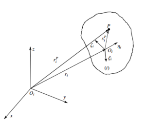
Figure 1: Cartesian Coordinate System

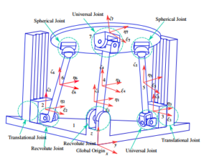
Figure 2: Global and Local coordinates of the parallel mechanism at the initial configuration

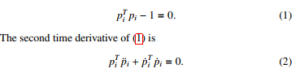
The parameter satisfies a mathematical relationship,

Denote R_i as a rotational matrix of body i, and a pair of 3×4 matrices

G_i and L_i defined as G_i = [−e,e˜ + e₀I]_i and L_i = [−e,−e˜ + e₀I]_i .

Then R_i = G_iL_i^T,[8] . The global coordinate of the point P illustrated in Figure 1 can be defined by

Denote q = q^T₁ ,q^T₂ ,q^T₃ ,q^T₄ ,q^T₅,q^T₆ ,q^T₇ as coordinate vector for describing the configuration of the mechanism, and its respective first and second time derivative, q˙ and q¨, for describing the motion of the mechanism. The number of coordinates of the system is n = 7 × 7 = 49, and the number of Euler parameters relationship (or mathematical constraint) is 7.

Denote

as kinematic equation derived from kinematic constraints which have 34 equations. The compact form of the kinematic equation for each joint is given in Appendix A. The first and second time derivative of (4) are written as

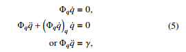
where γ = ⁻Φ_qq˙ q˙ is called the right side of the kinematic accelq eration equation and can be found in [8]. We adopt the constraint violation stabilization methods from [9], another similar technique can also be found in [10, 11].

Consider the following closed loop system,

where K_P and K_D are constant and defined in Appendix B. Due to the fact that there exists numerical errors in using numerical method to solve the differential equations (5), we use the positive constraint violation stabilization method to obtain a stable response. So (5) is modified such that the kinematic constraint equations are satisfied by ensuring the shrinking of the computation error.

First time derivative of constraint equation is obtained as

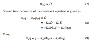
The equation (9) is used for simulation and the performance is discussed in section 5.

3. Dynamic Modeling for Unconstrained and Constrained Bodies

Newton-Euler equations of motion is used to derive the equations of motion for multi-rigid bodies of the parallel mechanism. Prior to having the equations of motion for a set of interconnected bodies by kinematic joints which is known as constrained body, the equations of motion for body with no contact to other bodies which refers as an unconstrained body are written.

3.1. Dynamic Equations for Unconstrained Bodies

From Newton’s method, an unconstrained body i with mass m_i and moment of inertia J_i⁰ with respect to its center of mass exerted by external force f_i and moment τ⁰_i has dynamic equation of motion as

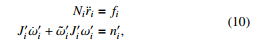
where N_i = diag m m m i and ω_i is the angular velocity defined in body-fixed frame. The equation of rotational motion in (10) is transformed by using the following relationships [8].

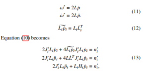
where H_i = 4L˙_i^T J_i^T L_i. The dynamic equations of motion for an unconstrained bodies are written as

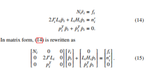
3.2. Dynamic Equations for Constrained Bodies

Bodies are interconnected to form a system of constrained bodies via kinematic joints which create constraint reaction forces and moments. When applying the constraint reaction forces and moments to (14), the dynamic equations of motion for a constrained bodies are written as

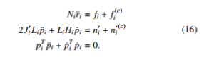
A constrained body i is additionally exerted by reaction forces and moments ^hf ^(c),n^0(c)iT from joints. These forces and moments can i be transformed to coordinate system consistent with q denoted by h ∗(c),n∗(c)iT and defined by f

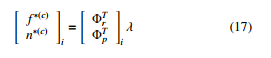
To be used with the formulation (16), the moment in (17) is transformed to be

where λ = [λ₁,…,λ₃₄] is known as Lagrange Multipliers, and

h             i

Φ_ri,Φ_pi = Φ_qi is Jacobian Matrix of the kinematic constraint Φ ≡ Φ(q) with respect to q_i. Therefore, the dynamic equations of motion for the mechanism are given in compact form as

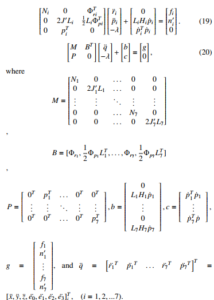
Equation (19) consists of 49 equations with 83 variables, therefore 34 constraint equations are appended with (19) to solve for coordinate vectors q and Lagrange multiplier λ. A system of algebraic differential equation is obtained as follow

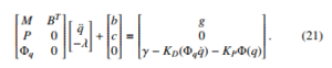
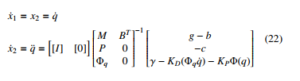
Equation (21) were solved for the coordinate vectors q by using state equations as follow:

x₁ = q = [x₁,y₁,z₁,[e₀,e₁,e₂,e₃]₁,…, x₇,y₇,z₇,[e₀,e₇,e₇,e₇]₇] x₂ = q˙ = [x˙₁,y˙₁,z˙₁,[e˙₀,e˙₁,e˙₂,e˙₃]₁,…, x˙₇,y˙₇,z˙₇,[e˙₀,e˙₁,e˙₂,e˙₃]₇] x˙₁ = x₂ = q˙

4. PD Controller

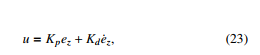
The desired value of actuator’s displacement is obtained from the 3D model such that the solar panel reach the position as shown in Figure 4 where the desired value of the two actuators are z_2d = 0.046m, z_2d = 0.046m . The actual displacement of the two actuators labeled as body number 2 and body number 3 are denoted as z₂ and z₃ respectively. Figure 3 illustrates a common feedback controller known as proportional derivative (PD) controller that is used to obtain the desired response, and has a form as follow:

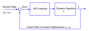
Figure 3: Block Diagram for PD Controller

where u =    , e_z =  and e˙_z = are the position f3z                     z3 − z3d      z˙3 − z˙3d

error and velocity error. K_p and K_d are 2 by 2 positive definite diagonal matrix. K_p plays a role as a spring that tries to keep the position error decreasing. K_d is considered as a damper which maintains the velocity error ˙e decreasing.

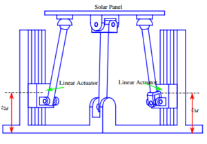
Figure 4: Desired configuration of the solar panel

5. Results and Discussion

PD control law is applied to drive the parallel mechanism from its initial configuration to the desired configuration with K_p =

”             #                        ”             #

50        0                             20      0

                   , and Kd =                               as shown in Figure 1 and Fig-

0         50                             0     25

h    i^T ure 4. The control input u =            f_2z                  f_3z                  is exerted to the two actuators by assigning the external forces in the vector g = h T             n10T              …             f7T                  n07TiT containing f1

while keeping the remaining components in g to be zero. Other parameters used in this paper are shown in Appendix C. As can be seen in the Figure 5, the two actuators reach the desired position quickly. The movement of the solar panel can be observed in Figure 7. It appears that the parallel mechanism can be easily controlled such that it is practically possible to move the solar panel directed to the sunlight, and thus more energy could be produced. It is evident that the desired orientation of the solar panel is with its coordinate system (ξ₇η₇ζ₇) is parallel to the global coordinate system (xyz). In this case, the euler parameters is expected to be

hφiT

equal to cos 0 0 sin ₂ [8], where φ is the rotation angle around ζ axis, and is reported true by Figure 8. Figure 9 illustrates the mathematical relationship of euler parameters of the solar panel as described in (1) which satisfies p^T₇ p₇ = 1. When the euler parameters are used to describe a rotational coordinate, it is important to ensure that (1) is satisfied because the four quantities of euler parameters are not independent.

6. Conclusion

Our study provides the frame work for modeling any mechanism by obtaining the algebraic differential equations of motion derived from Newton-Euler equation of motion and kinematic constraint equations. This technique can be applied to a wide range of simulation applications, especially for a close loop mechanism. Moreover, our result confirms the usefulness of the Baumgarte stabilization method that deals with numerical error when solving system of algebraic differential equations with mathematical constraint of Euler parameters. The control simulations using PD controller was to drive the solar panel to reach the desired configuration with a good performance.

Future work should focus on applying a model based controller that could provide a better control result, especially for tracking control. If the same modeling approach is applied to a system that requires fast response, an investigation on computation time should be made.

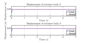
Figure 5: Response of Actuator’s Displacement

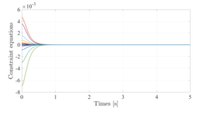
Figure 6: Kinematic constraint

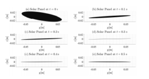
Figure 7: Orientation of Solar Panel

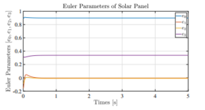
Figure 8: Euler Parameters Describing the Orientation of Solar Panel

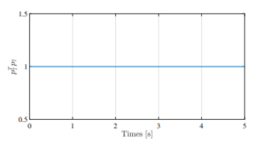
Figure 9: Mathematical Relationship of Euler Parameters of Solar Panel

APPENDIX A

For the parallel mechanism, by following the concept of relative constraints between two bodies from [8], the 34 constraint equations are obtained as follows:

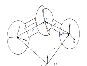
Figure 10: Spherical Joint

• Three equations for each Spherical joint between body (5,7) and

(6,7).

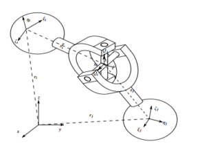
Figure 11: Universal Joint

• Four equations for each Universal joint between body (3,5) and (4,7).

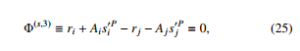
Figure 12: Revolute Joint

• Five equations for each Revolute joint between body (1,4) and

(2,6).

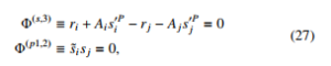
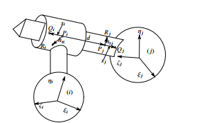
Figure 13: Translational Joint

• Five equations for each Translational joint between body (1,2) and (1,3).

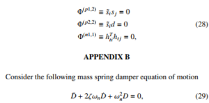
where ζ is a critical damping constant, and ω_n denotes a natural frequency. From (6) and (29), we can write

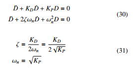
In the case of critically damped system, ζ = 1 ensures a fast response with no overshoot. Therefore, we choose K_D = 2α and K_P = α², where α is a positive constant and taken to be 10.

APPENDIX C

Table 1: Mass of body i,i = 1,2,··· ,7.

Symbols	Value	Unit
m1	475.09 × 10−3	Kg
m2	189.7 × 10−3	Kg
m3	189.7 × 10−3	Kg
m4	104.45 × 10−3	Kg
m5	53.25 × 10−3	Kg
m6	54.4 × 10−3	Kg
m7	890.5 × 10−3	Kg

Table 2: Position vector of center of mass of body i at initial position, i = 1,2,··· ,7

Symbols	Value	Unit
r1	10−3 × [−63.93,63.93,30.41]T	m
r2	10−3 × [−123.99,15,24.6]T	m
r3	10−3 × [−15,123.99,24.6]T	m
r4	10−3 × [−11.50,18.37,99.21]T	m
r5	10−3 × [−12.99,98.33,68.84]T	m
r6	10−3 × [−92.31,15,66.27]T	m
r7	10−3 × [−34.28,42.89,136.56]T	m

Table 3: Euler parameters of body i at initial position,i = 1,2,··· ,7

Symbols	Value
p1	[1,0,0,0]T
p2	[1,0,0,0]T
p3	[1,0,0,0]T
p4	[1,0,0,0]T
p5	[1,0,0,0]T
p6	[1,0,0,0]T
p7	[0.89043,−0.19791,−0.10481,0.39619]T

Table 4: Moment of Inertia of body i,i = 1,2,··· ,7

Symbols	Value						Unit
J10	 20  81 10−4 ×		8 20 1	−1 1 26			Kgm2
J20	 .2774 0 −0.00102 10−4 ×			0 0.2015 0	−0.0102 0 0.1987	 	Kgm2
J30	 .2015 0  00 10−4 ×			0 0.2774 0.0102	0.0102 0  0.1987		Kgm2
J40	 .1217 0 0.00000 10−3 ×			0.0000 0.1248 0	0  0 0.0054		Kgm2
J50	  10−4 ×	0.5827 0 −0.0824		0 0.5940 0	−0.0824 0 0.0172		Kgm2
J60	 .6242 0  00 10−4 ×			0 0.6231 −0.0000	−0.0000 0  0.0058		Kgm2
J70	 12  01 10−4 ×		0 12 0	1  0 24			Kgm2

Acknowledgment

This material is based upon work supported by the Air Force Office of Scientific Research under award number FA2386-17-1-0148.

1. S. Srang and S. Ath, “Dynamic Modeling and Simulation for 2DOF Parallel Mechanism Solar Tracker,” 2019 IEEE/ASME International Conference on advanced Intelligent Mechatronics (AIM), Hong Kong, China, 2019, pp. 283-288. https://doi.org/10.1109/AIM.2019.8868501
2. C.S. Chin, A. Babu, W. McBride, “Design, modeling and testing of a stan- dalone single axis active solar tracker using MATLAB/Simulink”, Renew- able Energy, Volume 36, Issue 11, 2011, Pages 3075-3090, ISSN 0960-1481. https://doi.org/10.1016/j.renene.2011.03.026
3. Yingxue Yao, Yeguang Hu, Shengdong Gao, Gang Yang, Jinguang Du, “A multipurpose dual-axis solar tracker with two tracking strategies”, Renewable Energy, Volume 72, 2014, Pages 88-98, ISSN 0960-1481. https://doi.org/10.1016/j.renene.2014.07.002
4. P. Y. Vorobiev, J. Gonzalez-Hernandez and Y. V. Vorobiev, “Optimization of the solar energy collection in tracking and non-tracking photovoltaic solar system,” (ICEEE). 1st International Conference on Electrical and Electronics Engineering, 2004., Acapulco, Mexico, 2004, pp. 310-314. https://doi.org/ 10.1109/ICEEE.2004.1433900
5. Hossein Mousazadeh, Alireza Keyhani, Arzhang Javadi, Hossein Mobli, Karen Abrinia, Ahmad Sharifi, “A review of principle and sun-tracking methods for maximizing solar systems output”, Renewable and Sustainable Energy Reviews, Volume 13, Issue 8, 2009, Pages 1800-1818, ISSN 1364-0321. https://doi.org/10.1016/j.rser.2009.01.022
6. T. Zhan, W. Lin, M. Tsai and G. Wang, “Design and Implementation of the Dual-Axis Solar Tracking System,” 2013 IEEE 37th Annual Com- puter Software and Applications Conference, Kyoto, 2013, pp. 276-277. https://doi.org/10.1109/COMPSAC.2013.46
7. J. Wu, X. Chen and L. Wang, “Design and Dynamics of a Novel Solar Tracker With Parallel Mechanism,” in IEEE/ASME Transactions on Mechatronics, vol. 21, no. 1, pp. 88-97, Feb. 2016. https://doi.org/10.1109/TMECH.2015.2446994
8. Nikravesh, Parviz E. Computer-aided analysis of mechanical systems, Prentice- Hall, Inc., 1988.
9. Neto, M.A., Ambro´sio, J. “Stabilization Methods for the Integration of DAE in the Presence of Redundant Constraints”. Multibody System Dynamics 10, 81–105 (2003). https://doi.org/10.1023/A:1024567523268
10. Flores, P., Machado, M., Seabra, E., and Tavares da Silva, M. (October 13, 2010). “A Parametric Study on the Baumgarte Stabilization Method for Forward Dynamics of Constrained Multibody Systems.” ASME. J. Comput. Nonlinear Dynam. January 2011; 6(1): 011019. https://doi.org/10.1115/1.4002338
11. Flores P., Pereira R., Machado M., Seabra E. (2009) “Investigation on the Baum- garte Stabilization Method for Dynamic Analysis of Constrained Multibody Systems”. In: Ceccarelli M. (eds) Proceedings of EUCOMES 08. Springer, Dordrecht.https://doi.org/10.1007/978-1-4020-8915-237

(Click Here)

(Click Here)