1. Introduction

A complete description of gas microflows involved in the micro/nano-electro-mechanical systems (MEMS/NEMS) [1] remains a challenge for many researchers during the last decades. Lid-driven cavity flow is one of the classical benchmark problems of computational fluid dynamics (CFD) [2–5]. Such flow has been analyzed by various computational methods like the Navier-StokesFourier equations (NSF) [6, 7], Direct Simulation Monte Carlo (DSMC) [7–10] and moment equations approach [6, 10, 11].

In micro-devices, gaseous flows undergoe non-equilibrium or rarefaction effects. The gas flow rarefaction degree is, usually, given by the Knudsen number (Kn) which is the ratio of gas-molecules mean free path (λ) and the characteristic length of the system (l) (see Fig. 1). The particle/wall collisions cease to be negligible against the particle/particle ones in the transition regime and the gas becomes rarefied. This situation takes place in many microfluidic and vacuum applications [12, 13].

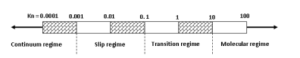
Figure 1: Flow regimes according to the Knudsen number.

To describe this kind of flows a kinetic based approach is needed. In order to save the computational time, the lattice boltzmann method (LBM) is used. This method was, first, inspired by the lattice gas automata (LGA) method for which the fluid is moving along the lattice. For both methods, the time, space, and velocities of the particles are discrete. The LGA model uses a six-speed hexagonal lattice, however, in LBM, the most used model for twodimensional (D = 2) geometries is D2Q9 which is a square grid with nine discrete velocities (Q = 9). In recent years, LBM has become a promising alternative to simulate fluid flows and heat transfer problems. Unlike the classical CFD approaches, the LBM is a mesoscopic approach which combines the classical computational fluid dynamics (CFD) and the kinetic description based on the Boltzmann equation. The method, therefore, ensures a relation between the macro and the microscopic descriptions of flow. Only a few studies that have investigated the effectiveness of this method and extend its ability to model hydrodynamic and rarefied flows [14–20]. However, the study of such flows requires a good choice and implementation of the boundary conditions (BC), which is a key step in the LBM simulation process. In the literature different BC are tested for various problems in order to capture non-equilibrium effects near the walls [21–25]. To solve the lattice Boltzmann equation (LBE), we used the well-known kinetic model of Bhatnagar–Gross–Krook (BGK) [26] which is the simplest and most widely used collision operator for the LBE. This operator is represented by a linear discretization of the relaxation of particle distribution function toward the Maxwell equilibrium state.

Application of LBM, under rarefaction conditions, to describe gas microflows is still a new field needing improvement to extend its applicability to this kind of flows. This study aims to simulate lid-driven gas flow in triangular micro-cavity. The results obtained by both approaches of LBM, SRT and MRT, are compared with those obtained by the DSMC method in the slip regime, usually encountered in MEMS devices [27]. The main simulation parameters are the Knudsen number (Kn) and the tangential momentum accommodation coefficient σ (TMAC). Unlike the DSMC method which needs a long computation time to give satisfactory results [28] and the extended macroscopic theory, like regularized 13 moment (R13), which the range of validity is limited [6, 29], the MRT-LBM proved its effectiveness for rarefied gas simulation.

2. Problem statement

In the current simulation, an isosceles right-angled triangular prism micro-cavity is considered with a large cross-sectional aspect ratio, the flow properties are independent of z-coordinate. In this study, the effect of any external body force is neglected. The gas flow can be considered within a two-dimensional enclosure of length scale H = L. According to the position of the moving wall, with a constant velocity U₀, two cases of the isosceles right triangle are considered in this study. In the first one, the right angle is in the topleft corner and the upper wall moves towards positive x-direction. However, in the second case, the right angle is in the bottom-left corner and the bottom wall moves in the negative x-direction (see Figs. 2).

3. Lattice Boltzmann models and boundary conditions

3.1. Boltzmann equation

Where f is the distribution function and Ω(f) is the collision operator which represents the particles microscopic collision dynamics.

In the BGK model, this operator is given by

In which τ represents the relaxation time and f ^eq is the Maxwell distribution function at the equilibrium state.

Figure 2: Studied domain configuration.

3.2. Single relaxation time lattice Boltzmann method (SRT-LBM)

For distribution function density f a D2Q9 model with square grid is used in this study. According to the BGK model, the governing, lattice Boltzmann equation, for this distribution function, is written as

The Maxwell distribution function f_k^eq at the equilibrium state is written in the Taylor expansion as

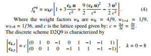
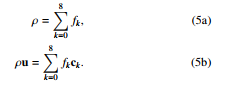
The macroscopic values of density ρ and velocity u = (u,v), are computed by the following relations:

For rarefied flows, the ratio of the mean free path λ and the

q

mean thermal velocity hvi = ^8RT_π is equivalent to the relaxation time τ given by

In microfluidic devices, gas flows are characterized by their rarefaction degree given by the Knudsen number Kn = _H^λ , where H is the total number of lattice nodes in the_√ y-direction. Usually, we

set c =      3RT = 1 for D2Q9 model, therefore [22]

3.3. Multi-relaxation time lattice Boltzmann method (MRT-LBM)

The collision operator in the multi-relaxation time lattice Boltzmann method (MRT-LBM) is given by

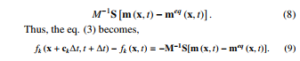
Where m(x,t) is a vector of moments and m^eq (x,t) is the corresponding one at the equilibrium state. The passage from the velocities space to the moments space and vice versa is obtained by the following linear transformations: m = Mf and f = M⁻¹m.

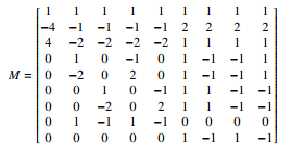
For D2Q9 scheme, the transformation matrix M is given by

The moments vector m is:

                 |mi = ρ     e    ε    ρu     q_x       ρv    q_y        p_xx          p_xy^T.

Where e is the energy, ε is the square of energy, j = (ρu,ρv) is the momentum of density, and q = (q_x,q_y) is the vector of heat flux.

The stress tensor components are also p_xx, and p_xy.

The moments vector at the equilibrium state m^eq (x,t) is given by

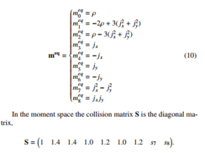
Where s₇ = s₈ = 1/τ. Note that by taking s_k = 1/τ, k = 0−8, the MRT model is reduced to the SRT one.

3.4. Stationary and moving walls boundary conditions

Boundary conditions implementation plays a crucial role in gas flow simulation within micro-geometries. In the present study, a combination of bounce-back and specular boundary conditions (BSBC) is used at the stationary walls, however, diffuse scattering boundary conditions (DSBC) are imposed at the moving wall.

• Combination of bounce-back and specular boundary conditions

The BSBC is adopted by using the coefficient of the tangential momentum accommodation σ (TMAC) expressed by [30]

Where M_i,r,w are the tangential momentum of molecules related, respectively, to the incident, reflected molecules, and wall. This coefficient ranges from 0 for pure specular reflection, to 1 which corresponds to the pure bounce-back one.

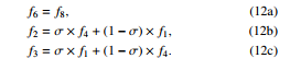
At the inclined wall, the boundary conditions using TMAC are as follows (see Fig. 3):

• Diffuse scattering boundary condition

The DSBC is used to simulate fluid interactions at solid interfaces written as [31]

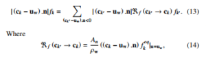
where k and k⁰ refer to the reflected and incident directions of molecules, respectively, and n is the unit normal vector inward of the wall, and <_f (c_k0 → c_k) is the scattering probability from the direction c_k0 to c_k. By satisfying zero normal flux condition across the wall, the coefficient of normalization A_n can be obtained by the following relation:

At the top wall, the unknown distribution functions are f_k=4/7/8

(see Fig. 3) can be determined from the known ones f_k=2/5/6 and

^f_k^eq_=4/7/8 as shown in the DSBC (Eqs. (13)–(15)) by

For the D2Q9 model, the coefficient A_n takes the value 6 [24].

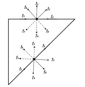
Figure 3: Gas-surface interaction at the top and inclined walls.

4. Results and discussion

All present simulations are carried out using a developed Fortran code. The SRT-LBM and MRT-LBM approaches are used to simulate lid-driven gas microflow in two configurations of triangular right micro-cavity isosceles (see Figs. 2). In the literature, the simulation of fluid microflows was made a lot for a square-section cavity [14–20]. However, a few studies were focused on the geometries with inclined sides [32–38]. Unlike most of these papers, based on the Reynolds number (Re), the rarefaction degree is expressed in this study according to the Knudsen number value (Kn).

4.1. Mesh independence study

For Kn = 0.01 and σ = 0.5, Table 1 shows mesh size effect on the x-velocity component at the center of the moving wall, while Figure 4 shows their effect on the profiles of u-velocity along the vertical line x/H = 1/3 and v-velocity along the horizontal line y/H = 2/3 for the case (1) using the SRT-LBM approach. Similarly, Figure 5 shows the profiles of u and v along the lines x/H = 1/3 and y/H = 1/3, respectively, for the case (2) by using the MRT-LBM approach. As shown, the grid size 300 × 300 is enough to offer good and reliable results.

Table 1: Effect of the mesh on the x-velocity component at the center of the moving

wall for Kn = 0.01 and σ = 0.5.

Mesh	200 × 200	300 × 300	400 × 400
SRT-LBM for case (1)	0.9120	0.9116	0.9115
MRT-LBM for case (2)	-0.9057	-0.9061	-0.9062

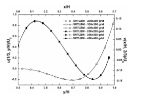
Figure 4: Profiles of u and v-velocity components along the lines x/H = 1/3 and y/H = 2/3, respectively, obtained by SRT-LBM for case (1).

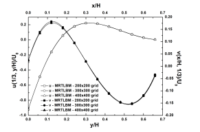
Figure 5: Profiles of u and v-velocity components along the lines x/H = 1/3 and y/H = 1/3, respectively, obtained by MRT-LBM for case (2).

4.2. Validation test

In order to ensure the validation of these models, a comparison is made with previous studies according to the widely used TMAC value (σ = 0.7) [14–16, 20] for both validation cases (square microcavity and a triangular micro-cavity (case(2)). At first, the profile of u−velocity for Kn = 0.01 and Kn = 0.1 along the vertical centerline are compared with the findings reported by Perumal et al. [14, 15] and Rahmati et al. [16] for a square micro-cavity (see Fig. 6a). Table 2 shows the location of the primary vortex center for Kn = 0.01 and

Kn = 0.1. The results of the current study align well with those of Rahmati et al. [16, 17], and Tang et al. [18]. In the second validation case, u-velocity contours inside a triangular micro-cavity (case (2)) are confronted with those obtained by the DSMC method [38], the most confident and powerful method to study of such flows. Figures 6b and 7 show, respectively, the u-velocity component profiles for x/H = 1/3 and the u contours for Kn = 0.01 and Kn = 0.1. Table 3 shows the location of the primary vortex center according to the Knudsen number values Kn = 0.01 and Kn = 0.1. It is shown that MRT-LBM results are acceptable and approximate well, those of Roohi et al. [38], for which U₀ = 100m/s.

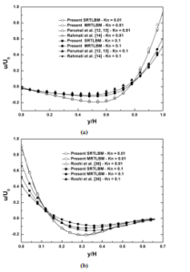
Figure 6: Profile of x-velocity for Kn = 0.01 and Kn = 0.1 (a) along the vertical centerline for square micro-cavity and (b) along the line x/H = 1/3 case (2) with a positive velocity +U₀.

4.3. Numerical results and analysis

In this work, the lid-wall moves with a fixed horizontal velocity U₀ = 0.1 for all simulations. To compare with and reproduce the results of Roohi et al. [38], the TMAC is taken σ = 0.7. Using the SRT-LBM and MRT-LBM methods, Figures 8 and 9 show the Knudsen number effect on the horizontal and vertical velocities profiles, respectively, for case (1) and case (2). The slip effect at the moving wall is more pronounced [14–17, 20, 38]. As predicted by the kinetic theory, the velocity slip vanishes at the continuum limit (Kn = 0.007), the gas-molecules velocity is almost equal the lid-velocity U₀. To evaluate both effects of rarefaction degree and TMAC value, Tables 4 and 5 show that as Kn and σ increase, the effects of non-equilibrium impact on the flow motion and the velocity slip evolve more importantly. For the first case, since the moving wall velocity is positive then the horizontal velocity component decreases to take negative values near the inclined wall, then increases to take positive values with y-coordinate beyond the primary vortex position. In that case, the lowest value of u/U₀ is located at y/H = 0.7 for Kn = 0.007 (see Figs. 8(a-b)). Similar and opposite behavior of u-component velocity is observed in the second case. The highest values of u/U₀ is located at y/H = 0.32 for Kn = 0.007

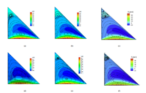
Figure 7: x-velocity streamlines and contours for σ = 0.7 – case (2) with a positive velocity +U₀. (a) SRT-LBM −Kn = 0.01 (b) MRT-LBM −Kn = 0.01 (c) Roohi et al. [38] −Kn = 0.01 (d) SRT-LBM −Kn = 0.1 (e) MRT-LBM −Kn = 0.1 (f) Roohi et al. [38] −Kn = 0.1.

Table 2: Primary vortex center locations for a square micro-cavity. Kn SRT-LBM MRT-LBM Rahmati et al. [16] Rahmati et al. [17] Tang et al. [18] 0.01 (0.5009,0.7638) (0.5030,0.76378) (0.5017,0.7637) (0.5022,0.7663) (0.5,0.7633) 0.1 (0.5001,0.7316) (0.5041,0.75336) (0.5020,0.7240) (0.5023,0.7570) (0.5,0.72) Table 3: Primary vortex center locations for the triangular micro-cavity (case (2)). Kn SRT-LBM MRT-LBM Roohi et al. [38] – Monatomic Roohi et al. [38] – Diatomic 0.01 (0.3979,0.1525) (0.3974,0.1523) (0.4209,0.1520) (0.4119,0.1520) 0.1 (0.3529,0.1888) (0.3678,0.1624) (0.3799,0.1659) (0.3780,0.1670)

(see Figs. 9(a-b)). The vertical velocity-slip increases when Kn increases and it is more prominent by the SRT-LBM approach than by the MRT-LBM one [16, 20] (see Figs. 8(c-d) and 9(c-d)). The MRT-LBM method maintains its stability near the walls and the vertical slip-velocity can be captured even at the center of the inclined plane on the right (see Figs. 10b and 10d). However, for the SRTLBM method, when the value of Kn increases fluctuations appear on and near the inclined wall. These fluctuations have a significant influence, especially for Kn = 0.1 (see Figs. 10a and 10c). For Kn = 0.01, 0.05, and 0.1, Table 6 shows the position of the primary and secondary vortices inside the micro-cavity for the first case. For both approaches, by increasing Kn, the primary vortex moves from right to left in the direction of x and from top to bottom in the direction of y. However, the secondary vortices at the bottom of the micro-cavity vanish and it cannot be captured using the SRT-LBM method while the MRT-LBM method retains their presence and these vortices undergo the same motion as the primary ones with Kn (see Figs. 12). For the value of TMAC σ = 0.7, these vortices are slightly shifted to the right with respect to the σ = 0.5 case. Table 7 presents the location of flow vortices in the second case. The primary vortex with Kn for both approaches moves from left to right in the direction of x and from bottom to top in the direction of y. But, SRT-LBM cannot retain its horizontal x-direction movement for Kn = 0.1. As in the case (1), unlike the SRT-LBM approach, the secondary vortices are well captured by MRT-LBM. These vortices move as the primary one along y-direction but in the opposite x-direction. Thus, unlike in the square-cavity, in the presence of an inclined wall, the flow stagnation points undergo two motion under rarefaction effects. For σ = 0.7, both types of vortices are moved in downward direction and shifted to the right with respect to the σ = 0.5 case. For different Knudsen numbers, the flow stagnation which corresponds to u/U₀ profiles intersection point remains the same (see Table 8, Figs. 8 (a-b) and Figs. 9(a-b)). The density ρ is also sensitive to the rarefaction degree and its value increases with Kn. An expected density has a great value near the upper-right and lower-left corners, for the cases (1) and (2), respectively (see Fig. 11a). To examine the required run time for both approaches, the profiles of velocity components at the gravity center of the micro-cavity (1) (x = H/3,y = 2H/3) are plotted as a function of the number of time steps for Kn = 0.01 and σ = 0.7. After approximately 10000time steps number the velocity hits the steady-state (see Figs. 11b and 11c). Developed codes SRT-LBM and MRT-LBM are run on the Intel (R) Core (TM) i5-3340 M CPU laptop @ 2.7 GHz and RAM 8.00 GB. To obtain accurate findings the MRT-LBM requires more processing time than the SRT-LBM [16, 20] due to the higher number of moments hired in the calculation to capture the effects of non-equilibrium (see Table 9). In Figures 12(a-i) the flow streamlines and u-velocity contours are plotted for Kn = 0.007, 0.05, 0.1, 1 and 3, respectively for σ = 0.7. As the increase in the Knudsen number, the streamlines take the wall shape and the secondary vortices observed for the lower Knudsen numbers vanish at the bottom of the micro-cavity (1) [14–16, 20]. In addition, the primary vortex undergoes a slight downward, and right-to-left movement with Kn growth. Also, u-velocity is sensitive to the degree of rarefaction and its value decreases as Kn increases. Figures 13 describe the flow streamlines, u and v-velocities contours for Kn = 0.007 and Kn = 0.1, respectively, by combining the cavity of case(1)/case(2) with their corresponding anti-symmetric cases. The segments connecting the primary and secondary vortices centers intersect at the center of the square micro-cavity, respectively (see Figs. 13(a-b)). The plots of the velocity components distributions, Figures 13(c-f), confirm the data anti-symmetric variation with respect to the square cavity center and their sensitivity to the rarefaction effect. So, by studying the two cases (1) and (2) we can deduce the characteristics of the gas flow in their corresponding anti-symmetrical forms.

Finally, it is shown that SRT-LBM loses its validity in the transition regime while the results of the MRT-LBM method still remain convincing. To summarize the MRT-LBM method imposes itself as a good alternative for simulating the gas microflows usually encountered in the micro-devices.

Table 4: Slip effects on the x-velocity component u (HU/20,H) at the center of the moving wall – case (1).		Table 5: Slip effects on the x-velocity component u (HU/02,0) at the center of the moving wall – case (2).
Approaches Kn 0.007       0.01        0.05          0.1	Approaches Kn 0.007         0.01          0.05           0.1
SRT-LBM σ = 0.5 0.9372 0.91165 0.64171 0.41041 σ = 0.7 0.93674 0.91076 0.63227 0.39725 MRT-LBM σ = 0.5 0.93739 0.91214 0.67381 0.51394 σ = 0.7 0.93692 0.91126 0.66554 0.50135	SRT-LBM σ = 0.5 -0.93045 -0.90587 -0.63838 -0.41238 σ = 0.7 -0.92999 -0.90498 -0.62877 -0.39784 MRT-LBM σ = 0.5 -0.93042 -0.90617 -0.67291 -0.51524 σ = 0.7 -0.92998 -0.90531 -0.66484 -0.50287

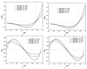
Figure 8: (a)-(b) x-velocity profile along the vertical line x/H = 1/3 and (c)-(d) profile of y-velocity along the horizontal line y/H = 2/3 at different Knudsen numbers for σ = 0.7 – case (1).

Table 6: Primary and secondary vortices locations for different values of Kn and σ – case (1).

SRT-LBM (σ = 0.5) MRT-LBM	Primary vortex         (0.3939,0.8455) (0.3697,0.8298) (0.3493,0.8035) Secondary vortex (0.0770,0.2711)          − − − − −                − − − − −
	Primary vortex         (0.3933,0.8458) (0.3681,0.8360) (0.3660,0.8298) Secondary vortex (0.1101,0.2572) (0.0884,0.1807)            − − − − −
SRT-LBM (σ = 0.7) MRT-LBM	Primary vortex         (0.3944,0.8471) (0.3713,0.8351) (0.3526,0.8106) Secondary vortex (0.0783,0.2821)          − − − − −                − − − − −
	Primary vortex         (0.3938,0.8473) (0.3702,0.8416) (0.3681,0.8377) Secondary vortex (0.1124,0.2669) (0.1018,0.2293) (0.0910,0.1878)

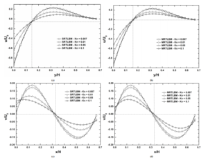
Figure 9: (a)-(b) x-velocity profile along the vertical line x/H = 1/3 and (c)-(d) profile of y-velocity along the horizontal line y/H = 1/3 at different Knudsen numbers for σ = 0.7 – case (2).

Table 7: Primary and secondary vortices locations for different values of Kn and σ – case (2).

SRT-LBM (σ = 0.5) MRT-LBM	Primary vortex         (0.3275,0.1616) (0.3514,0.1709) (0.3379,0.1944) Secondary vortex (0.0871,0.7438)          − − − − −                − − − − −
	Primary vortex         (0.3272,0.1612) (0.3508,0.1653) (0.3537,0.1709) Secondary vortex (0.1069,0.7517) (0.0879,0.8217)            − − − − −
SRT-LBM (σ = 0.7) MRT-LBM	Primary vortex         (0.3296,0.1597) (0.3539,0.1653) (0.3404,0.1870) Secondary vortex (0.0896,0.7329)          − − − − −                − − − − −
	Primary vortex         (0.3293,0.1594) (0.3536,0.1596) (0.3555,0.1630) Secondary vortex (0.1098,0.7417) (0.1020,0.7727) (0.0912,0.8133)

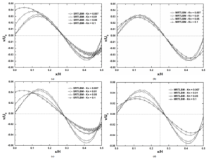
Figure 10: Profile of y-velocity along the horizontal line y/H = 0.5 at different Knudsen numbers for σ = 0.7 (a) SRT-LBM – case (1) (b) MRT-LBM – case (1) (c) SRT-LBM – case (2) and (d) MRT-LBM – case (2).

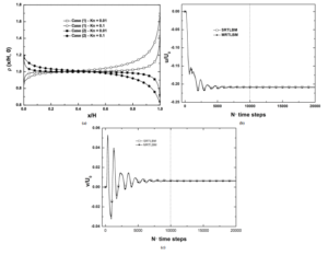
Figure 11: For σ = 0.7. (a) Density along the moving wall for Kn = 0.01 and Kn = 0.1 for both cases by using the MRT-LBM method and (b)-(c) Evolution of x and y-velocities at the center of gravity of the micro-cavity as a function of time for Kn = 0.01 by using both methods – case(1).

Table 8: Coordinates (y/H,u/U₀) of the common intersection points at the line x/H = 1/3 for σ = 0.7.

SRT-LBM	(0.874,0.094)	(0.145, −0.005)
MRT-LBM	(0.866,0.064)	(0.159, −0.004)

Table 9: Execution time for 1000 iterations.

SRT-LBM	10.4s	21.4s	37.3s
MRT-LBM	30.8s	65.4s	113.3s

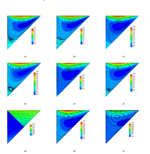
Figure 12: The flow streamlines and x-velocity contours for σ = 0.7 (case (1)) (a) SRT-LBM −Kn = 0.007 (b) MRT-LBM −Kn = 0.007 (c) SRT-LBM −Kn = 0.05 (d) MRT-LBM −Kn = 0.05 (e) SRT-LBM −Kn = 0.1 (f) MRT-LBM −Kn = 0.1 (g) SRT-LBM −Kn = 1 (h) MRT-LBM −Kn = 1 and (i) MRT-LBM −Kn = 3.

Figure 13: The flow streamlines, x and y-velocities contours for σ = 0.7, respectively. (a, c and e) SRT-LBM −Kn = 0.007 (case (1) with its corresponding anti-symmetric shape) and (b, d and f) MRT-LBM −Kn = 0.1 (case (2) with its corresponding anti-symmetric shape).

5. Conclusion

In the current paper, a comparison between SRT-LBM and MRT-LBM confirms MRT-LBM method’s ability to simulate rarefied gas flows. A lid-driven flow inside an isosceles triangular cavity is investigated numerically. The range of Knudsen numbers discussed is from the slip to the early transition regime. To capture non-equilibrium effects near the walls slip boundary conditions are used. It is clear that the SRT-LBM loses its validity with increasing the rarefaction degree while the MRT-LBM findings approximate well with those obtained by the DSMC method. To sum up, this research reveals many interesting characteristics of micro lid-driven microflows. In the slip regime, for small values of the Knudsen number, the results demonstrate that both methods are good alternatives, but in the transition regime, only MRT-LBM shows its capability to describe the gas microflows usually found in the MEMS/NEMS devices.

Nomenclature

H, L         Cavity height and length

t              Time

Kn           Knudsen number

Re             Reynolds number R   Gas constant c          Lattice speed c_s             Speed of sound

c_k                     Lattice velocity vector u             Velocity vector U₀        Velocity of the moving wall f      Density distribution function f_eq Equilibrium density distribution function w_k Weight factors in the equilibrium distribution M          Transformation matrix for D2Q9 scheme

m           Moment vectors

m^eq              Equilibrium moment vectors

S             Collision matrix

Greek Symbols

λ            Mean free path

∆t           Time step

∆x, ∆y      Lattice spacing in x and y directions

τ              Momentum relaxation time σ    Tangential Momentum Accommodation Coefficient (TMAC)

ρ             Density

Conflict of Interest

The authors declared no potential conflicts of interest with respect to the research, authorship and publication of this article.

Acknowledgments

The authors wish to express their cordial thanks to the Editors and Reviewers for their valuable suggestions and constructive comments whish have served to improve the quality of this paper.

Funding

The authors received no financial support for the research, authorship and publication of this article.

1. M. Gad-El-Hak, “The fluid mechanics of microdevices—the freeman scholar lecture,” Journal of Fluids Engineering, Transactions of the ASME, 121(1), 5–33, 1999, doi:10.1115/1.2822013.
2. U. Ghia, K. N. Ghia, C. Shin, “High-Re solutions for incompressible flow using the Navier-Stokes equations and a multigrid method,” Journal of computational physics, 48(3), 387–411, 1982, doi:10.1016/0021-9991(82)90058-4.
3. K. Ghasemi, M. Siavashi, “Three-dimensional analysis of magnetohydrody- namic transverse mixed convection of nanofluid inside a lid-driven enclosure using MRT-LBM,” International Journal of Mechanical Sciences, 165, 105199, 2020, doi:10.1016/j.ijmecsci.2019.105199.
4. A. Bo, F. Mellibovsky, J. Bergada`, W. Sang, “Towards a better understanding of wall-driven square cavity flows using the lattice Boltzmann method,” Applied Mathematical Modelling, 82, 469–486, 2020, doi:10.1016/j.apm.2020.01.057.
5. T. Huang, H.-C. Lim, “Simulation of Lid-Driven Cavity Flow with Inter- nal Circular Obstacles,” Applied Sciences, 10(13), 4583, 2020, doi:10.3390/ app10134583.
6. J. Baliti, M. Hssikou, M. Alaoui, “Rarefaction and external force effects on gas microflow in a lid-driven cavity,” Heat Transfer—Asian Research, 48(1), 80–99, 2019, doi:10.1002/htj.21369.
7. S. Mizzi, D. R. Emerson, S. K. Stefanov, R. W. Barber, J. M. Reese, “Effects of rarefaction on cavity flow in the slip regime,” Journal of computational and theoretical nanoscience, 4(4), 817–822, 2007, doi:10.1166/jctn.2007.2374.
8. A. Mohammadzadeh, E. Roohi, H. Niazmand, “Simulation of Rarefied Gas Flow in Micro/Nano Cavity Using DSMC,” in 10th Iranian Aerospace Society Conference, 2011.
9. B. John, X.-J. Gu, D. R. Emerson, “Investigation of heat and mass transfer in a lid-driven cavity under nonequilibrium flow conditions,” Numerical Heat Transfer, Part B: Fundamentals, 58(5), 287–303, 2010, doi:10.1080/10407790. 2010.528737.
10. A. Mohammadzadeh, A. Rana, H. Struchtrup, “DSMC and R13 modeling of the adiabatic surface,” International Journal of Thermal Sciences, 101, 9–23, 2016, doi:10.1016/j.ijthermalsci.2015.10.007.
11. A. Rana, M. Torrilhon, H. Struchtrup, “A robust numerical method for the R13 equations of rarefied gas dynamics: Application to lid driven cavity,” Journal of Computational Physics, 236, 169–186, 2013, doi:10.1016/j.jcp.2012.11.023.
12. G. A. Bird, J. Brady, Molecular gas dynamics and the direct simulation of gas flows, volume 5, Clarendon press Oxford, 1994.
13. F. Sharipov, Rarefied gas dynamics: fundamentals for research and practice, John Wiley & Sons, 2015.
14. D. A. Perumal, G. V. Kumar, A. K. Dass, “Application of Lattice Boltzmann Method to Fluid Flows in Microgeometries.” CFD letters, 2(2), 2010.
15. D. A. Perumal, V. Krishna, G. Sarvesh, A. K. Dass, “Numerical Simulation of Gaseous Microflows by Lattice Boltzmann Method,” International Journal on Production and Industrial Engineering, 2(1), 11, 2011.
16. A. Rahmati, S. Niazi, “Application and comparison of different lattice Boltz- mann methods on non-uniform meshes for simulation of micro cavity and micro channel flow,” Computational Methods in Engineering, 34(1), 97–118, 2015, doi:10.18869/ACADPUB.JCME.34.1.97.
17. A. Rahmati, S. Niazi, “A multi relaxation time lattice Boltzmann method for simulation of flow in micro devices,” in Proc. 19th Annual Int. Conf. on Mechanical Engineering, Birjand, Iran, 2011.
18. G. Tang, W. Tao, Y. He, “Lattice Boltzmann method for gaseous microflows using kinetic theory boundary conditions,” Physics of Fluids, 17(5), 058101, 2005, doi:10.1063/1.1897010.
19. G. Tang, W. Tao, Y. He, “Simulating two-and three-dimensional microflows by the lattice Boltzmann method with kinetic boundary conditions,” Interna- tional Journal of Modern Physics C, 18(05), 805–817, 2007, doi:10.1142/ S0129183107010577.
20. Y. Elguennouni, M. Hssikou, J. Baliti, R. Ghafiri, M. Alaoui, “SRT-LBM and MRT-LBM comparison for a lid-driven gas microflow,” in 2020 1st Interna- tional Conference on Innovative Research in Applied Science, Engineering and Technology (IRASET), 1–6, IEEE, 2020, doi:10.1109/IRASET48871.2020. 9092233.
21. X. Nie, G. D. Doolen, S. Chen, “Lattice-Boltzmann simulations of fluid flows in MEMS,” Journal of statistical physics, 107(1-2), 279–289, 2002, doi:10.1023/A:1014523007427.
22. C. Lim, C. Shu, X. Niu, Y. Chew, “Application of lattice Boltzmann method to simulate microchannel flows,” Physics of fluids, 14(7), 2299–2308, 2002, doi:10.1063/1.1483841.
23. G. Tang, W. Tao, Y. He, “Thermal boundary condition for the thermal lat- tice Boltzmann equation,” Physical Review E, 72(1), 016703, 2005, doi: 10.1103/PhysRevE.72.016703.
24. X. Niu, C. Shu, Y. Chew, “Numerical Simulation of Isothermal Micro Flows by Lattice Boltzmann Method and theoretical analysis of the Diffuse scatter- ing boundary condition,” International Journal of Modern Physics C, 16(12), 1927–1941, 2005, doi:10.1142/S0129183105008448.
25. Q. Zou, X. He, “On pressure and velocity boundary conditions for the lat- tice Boltzmann BGK model,” Physics of Fluids, 9(6), 1591–1598, 1997, doi: 10.1063/1.869307.
26. P. L. Bhatnagar, E. P. Gross, M. Krook, “A model for collision processes in gases. I. Small amplitude processes in charged and neutral one-component systems,” Physical review, 94(3), 511, 1954, doi:10.1103/PhysRev.94.511.
27. G. Karniadakis, A. Beskok, N. Aluru, Microflows and nanoflows: fundamentals and simulation, volume 29, Springer Science & Business Media, 2006.
28. M. Hssikou, J. Baliti, Y. Bouzineb, M. Alaoui, “DSMC method for a two- dimensional flow with a gravity field in a square cavity,” Monte Carlo Methods and Applications, 21(1), 59–67, 2015, doi:10.1515/mcma-2014-0009.
29. M. Hssikou, J. Baliti, M. Alaoui, “Extended macroscopic study of dilute gas flow within a microcavity,” Modelling and Simulation in Engineering, 2016, 2016, doi:10.1155/2016/7619746.
30. Y. Zhang, R. Qin, Y. Sun, R. Barber, D. Emerson, “Gas flow in microchannels– a lattice Boltzmann method approach,” Journal of Statistical Physics, 121(1-2), 257–267, 2005, doi:10.1007/s10955-005-8416-9.
31. S. Ansumali, I. V. Karlin, “Kinetic boundary conditions in the lattice Boltzmann method,” Physical Review E, 66(2), 026311, 2002, doi:10.1103/PhysRevE.66. 026311.
32. E. Erturk, O. Gokcol, “Fine grid numerical solutions of triangular cavity flow,” The European Physical Journal Applied Physics, 38(1), 97–105, 2007, doi: 10.1051/epjap:2007057.
33. F. Munir, N. A. Che Sidik, M. Rody, H. Zahir, M. Tahir, “Numerical simula- tions of shear driven square and triangular cavity by using Lattice Boltzmann scheme,” World Academy of Science, Engineering and Technology, 70, 190– 194, 2010.
34. F. A. Munir, M. I. M. Azmi, M. R. M. Zin, M. A. Salim, N. A. C. Sidik, “Ap- plication of lattice Boltzmann method for lid driven cavity flow,” International Review of Mechanical Engineering, 5(5), 856–861, 2011.
35. M. Idris, C. Nor Azwadi, N. N. Izual, “Vortex structure in a two dimensional triangular lid-driven cavity,” in AIP Conference Proceedings, volume 1440, 1078–1084, American Institute of Physics, 2012, doi:10.1063/1.4704323.
36. M. Nazari, “LBM for modeling cavities with curved and moving boundaries,” Modares Mechanical Engineering, 13(5), 117–129, 2013.
37. B. An, J. M. Bergada` Granyo´, “Numerical study of the 2D lid-driven triangu- lar cavities based on the Lattice Boltzmann method,” in Proceedings of the 3rd Annual International Conference on Mechanics and Mechanical Engineer- ing:(MME 2016), 945–953, Atlantis Press, 2016, doi:10.2991/mme-16.2017. 133.
38. E. Roohi, V. Shahabi, A. Bagherzadeh, “On the vortical characteristics and cold-to-hot transfer of rarefied gas flow in a lid driven isosceles orthogonal triangular cavity with isothermal walls,” International Journal of Thermal Sciences, 125, 381–394, 2018, doi:10.1016/j.ijthermalsci.2017.12.005.

(Click Here)

(Click Here)