1. Introduction

Most of the cybersecurity issues are related to malware. Malware is malicious software. The first malware, “Morris worm” which is also a virus appeared in 1989-90. Malware is used to collect personal, financial data of a user and give control of ICT (Information Communication Technology) devices mobiles, computers, and systems to command and control centers managed by hacker groups. Malware is at the helm of the cybersecurity issue. The goal of hacker groups or hackers is to make the malware reach the system, network gear, and then use it for their ulterior motives. It may cost millions of dollars if one malware goes undetected [1]. As society becomes increasingly dependent on the computing system, it is important to detect malicious software (Malware). Specific code sequences, signature, executed by a virus are used by antivirus to detect the malware. Finding such code sequences is not matching with the speed at which new malware is being generated with greater use of ICT systems in varieties of areas ranging from individual, business, industrial. Nowadays with the Internet of Things (IoT), Industry 4.0, the use of ICT has grown at a very large rate and so has the attraction of hackers to hack them by use of malware, software with disingenuous intention, such as virus, worm, rootkit, key logger, Trojan horse, ransomware, spyware, etc. To detect this malware using traditional methods such as using a signature base [2] will leave much malware undetected, resulting in security issues. A signature-based approach is used in antivirus software. A signature is set with static and/or dynamic analysis manually to identify the malware. Malware authors keep the same functionality but polymorph the malware. Such polymorphed malware cannot be detected by antivirus as the signature is different. This problem is currently rampant. New polymorphed malware can be detected by a machine learning approach. The signature-based approach is insufficient as millions of new malware appear almost on an everyday basis. A technique needs to be developed that generalizes to new malware. Hence, detection of malware using machine learning is the right choice. Efficient automated malware detectors are required to classify software, application as malware, or benign.

The dataset for malware research is not available publicly due to privacy concerns. Few online databases of malware [3] allow limited use of data. Many malware detection research is done using unbalanced data, the number of malware is very high compared to benign software. There may be discrepancies in malware data collected and that may be possible in a real environment. For effective malware research, one needs the large, balanced recent, and right mix of families of malware database [4]. With a large database with many attributes related to malware, one needs to use expensive, complex, and high-end computing machines. In this research, we plan to use one such large database [5], which is shared publicly and low computing resources to build a matching or better malware detection system. Here we aim at extracting low dimension, effective features that contribute to learning and result in effective classifiers to detect malware. XGboost using Gradient Boost Decision Tree (GBDT) algorithm is used to extract few effective features from a large database with large attributes.  To our knowledge, the complete dataset is not used with the XGboost GDBT algorithm. We use this combination to extract the features, which can be used with low-end computing resource to build effective malware classifier.  This paper is organized with a background related to malware detection in section 2, the literature survey in section 3, methodology in section 4, experiments, and results in section 5, and conclusion in section 6.

2. Background

For malware, detection features may be extracted from the file format they are packed in. The executable, libraries, objects are packed using Common Object File Format (COFF). For the Windows operating system, it is Portable Executable 32/64 (PE32/64) [6,7].  It may also be possible to find file agnostic features such as histogram of bytes in the program, byte entropy of various parts of a program [8], or strings available in the program [9]. The string may include URL accessed, registry accessed, deleted, modified, or files accessed, deleted or modified or IP address accessed, files accessed, created, deleted and modified, registry created, modified, and deleted. It may be possible to find a set of features for the detection of malware. A neural network can help achieve a higher-level representation of malware. The sequence classifier takes n bytes, n-gram, as input in [10]. However, it is limited to a few bytes or kilobytes. However, for malware, it may have to take millions of bytes, as the size of executable programs. The efficient extraction of features leads to efficient malware detection. Deep learning models use a complete executable without the need for features from domain knowledge [11]. It takes high-end computing resources and a large amount of time.

2.1. Portable executable

Windows binary consists of PE header [6], code, data, and resource part. The PE header has a COFF Header, optional header, and section tables. Each of these has subparts and further subparts. COFF header consists of 24 bytes and has signature 0x50450000, Machine, Number of sections, TimeDate. The Optional header has a standard COFF field of 28 bytes, windows specific field of 68 bytes, and data directories of 144 bytes data directories. The standard COFF consists of magic, major, minor linker version, size of code, initialized data, uninitialized data, address of entry point, the base of code, data, etc. Windows-specific field consists of image base, section, file alignment, major, minor OS version, major, minor image version, major, minor subsystem version, win32 version value, size of image, header, checksum, subsystem, DLL characteristics, size of stack reserved, commit, size of heap reserve, commit, loader flags, number of RVA and sizes. The data directory consists of various table and size of tables such as location and size Export table, Import table, Resource table, Exception table, Certificate table, Base relocation table, Debug, architecture data, TLS table, Load Config, Bound Import, Import Address Table (IAT), Delay import descriptor, CLR runtime header, Global ptr. Each of the section tables consists of 40 bytes and contains information such as name, Virtual size, and address, location, and size of Raw data, Number of relocations, Number of line number, characteristics. There may be more than one section. Name of sections are .text, .rdata, .data, .idata, .rsro, .rsrc etc. There are several methods to extract these fields. The technique employed here is to use LIEF (Library for Instrumenting Executable Files) [12].

2.2. Techniques used for malware detection

Malware can be detected using a static or dynamic detection method. The Static method [13,14] identifies the malware before the execution of the file and serves as a critical defense mechanism. Static malware detection does not execute the malware and uses the structural information as file format [6, 15] available in applications. One has to identify efficient features to be used to build malware detection systems. If we get information from a binary program using techniques such as Portable Executable 32/64 (PE32/64) header information for windows program. Polymorphic, Metamorphic malware is created by malware authors with minor changes to avoid detection by antiviruses, which uses signature-based detection. In Polymorphism, the malware authors use a combination of data prepend, data append, and encryption, decryption to generate malware in large numbers. In metamorphism, the malware themselves change code by a combination of dead code, code transposition, register reassignment, and instruction substitution can generate a large amount of malware. As the signature changes in polymorphic malware, the antivirus is unable to detect malware. As malware authors use various means to avoid detection such as obfuscated code [16], convoluted systems library calls, detection of malware has a limitation. At times, code is obfuscated by non-standard, private methods [7,16] to make the detection more difficult even by domain experts. Such complexity in detection may be avoided by dynamic malware detection [17-19].

In dynamic malware detection, the application is allowed to run in a protected virtual environment. The application unfolds all the obfuscation, convoluted means of making systems call, and the effects of malware can be observed. For dynamic analysis, the malware cannot be executed on a normal system, as it will infect the system. It has to be run in a sandbox or special customized virtual environment to restore the system to a previous state when the malware was not run. The computational needs are high in a virtual environment or machine. Malware author builds features in malware to detect such a virtual machine environment. Once the malware detects such a virtual environment, the malware changes its behavior and behaves as normal benign software. There have been efforts to avoid the detection of the virtual environment by malware [20, 21]. An expert may declare such malware as benign, which causes unprecedented destruction, loss in a real normal working environment. The dynamic malware detection uses effects caused by malware such as files created, modified, deleted, or registries created, modified, deleted, or network connection set up to specific IP addresses to command and control centers of malware authors or to download next set of malware. It is time-consuming to run the malware in a virtual environment and observe the effects of each malware. Doing this exercise for a large number of malware generated these days due to polymorphism and metamorphism requires a large time and a large number of domain experts. In addition to the challenge of changing the behavior of malware on detection of the virtual environment, both time and domain experts are not available. Hence, it emphasizes the use of deep learning and machine learning techniques for malware detection.

Deep learning [11, 22-25] and machine learning [5,10, 26-29] has been used to make automated detectors to identify the malware and the family of malware. In most cases dataset used [26] are not available, unbalanced or detectors work with an unavailable specific setting and specific datasets. A private emulation environment is required to overcome challenges imposed by dynamic analysis. It also makes it difficult, as a private, non-public environment is not available. As the data and the parameters used for building models are not available, it is not possible to compare the results, accuracies across the works. Our work uses the open dataset [5]. It is a balanced dataset with 300k malware, 300k benign applications with 2351 hashed features [28,30] derived using LIEF [12] and portable executable file format [6] for training and separate 100k malware and 100k benign software with the same number of hashed feature sets for testing. The statistical summary of benign files is used to reduce the privacy concern. SVM with nonlinear kernel needs O(N**2) multiplication for one iteration. N is the number of samples in the dataset. K-NN needs not only computation at the same level but also all the labels in memory. Hence, these methods are not scalable. Scalable alternatives are the neural network, ensemble decision tree. The ensemble algorithm has been effective with large samples and features. Gradient Boosting Decision Tree (GBDT) algorithm used in XGboost [31, 32], LightGBM [33,34] will be more effective for large dataset with large feature sets. There are multiple times, maybe twenty-plus, improvement in the training process.

3. Literature survey

In [17] author used a list of Dynamic Link Library (DLL) from the PE header and list of functions imported from those DLL as features. Besides, they used few more PE header features as well on a dataset of 4206 samples. It had 3265 malware. They achieved a 97.76 % detection rate. In [13], PE Miner framework, author used 189 features consisting of section size, features from the COFF section, resource table, and import of DLL as binary features. All the features were derived from the PE header. Specific DLL group’s functions used for a specific purpose and import of DLL indicates the intent of the software. They achieved the Area Under Curve (AUC) of .991 and False Positive (FP) rate < 0.5% for on dataset of 15000 samples. In [35] author used a dataset of 116000 samples consisting of 100000 malware and remaining benign software. They started with 100 features from the PE header and iterated to finalize of 7 most influencing features. It is also termed as Adobe malware classifier. They achieved a TP rate of 98.56% and an FP rate of 5.68% on 1/5th of the dataset using tenfold cross-validation. The High FP rate is also reported in [5] by using the specified 7 features from the PE header. In [36], SAVE (Static Analyzer of Vicious Executables), author  use the API calling sequence of specific identified packed obfuscated malware to find similarity measures with other samples to detect malware. They use Euclidean distance to generate similarity report and detect new malware as one of the families of malware compared with. They use a 32-bit vector consisting of DLL name as 16 bit and each API in a DLL as another 16 bits.

In [37] author extract the behavior attributes of 10 different families of ransomware aggregating to 150 samples. Three different machine learning algorithms J48 Decision tree, KNN, Naive Bayes are used for classification. They use Virustotal [3] to get the behavioral report of each ransomware sample. It is like getting features and their value using the dynamic analysis. They achieve a classification accuracy of 78% by reducing the number of attributes to 12 from 27. In [18] author extract API calls of malware by dynamic analysis method and use fours step methodology to determine suspicious behavior. The suspicious behavior is identified by copy, delete, search, move, read, write, and change attributes operations on a file. They use calling sequence and statistical analysis to identify the malware. 386 samples are used of which 77% were packed using Armadilo, UPX, PE lock, Upack, KKrunchy. In [38] author use Hidden Markov Model using API calls and opcode. All combinations of static and dynamic analysis for the training phase and test phase are experimented such as static analysis data for training and static analysis data for testing, static analysis data for training, and dynamic analysis data for testing. They use 745 malware samples from 6 families of malware and report various AUC-ROC and AUC-PR (Area Under Curve – Precision-Recall) results. In [24], MtNet (A multi-task neural network), author use an anti-malware engine to extract the sequence of API and parameters used in those API and null-terminated objects from system memory. They believe the majority of null-terminated objects are unpacked strings and indicate a code fragment of malware. Many events to one event mapping are performed considering multiple API achieve the same results. Besides API trigram is made for three API calls. 50,000 feature sets are reduced to 4,000 and random projection is used to further reduce the training time of the neural network. Very large size database of 6.5 Million samples used in this project. It has a training data sample of 4.5 million consisting of 1.3 Million malware from 98 families, 1.55 Million generic malware, and 3.65 benign software. The test data is separate 2 Million samples. They experiment with the effects of hidden layers on accuracy and report an accuracy of 99.51% and low FP and FN rate. In [39] author uses dynamic analysis and CNN to build classifiers using 9 families of malware, each with 1000 malware. They achieve 99% Precision, Recall, and F1 score and FPR of 1%. Malware variants of one family have the same type of API calling sequence. Hence, feature image build using color-coding resembles and this similarity of the image is detected using CNN.

In [40] author  uses malware image fingerprints using the concept of GIST – Global Image Descriptor to compact image features and store malware in a large database of 4.3 million malware. New malware is pre-processed to compact image features as done with each of the malware in the database and search the database for in 3 seconds to find the matching image. In [41] author used 8 bits of a byte of executable a vector for building a greyscale image of fixed width. Image visualization of the binary value of executable gives more information about different sections and structures of malware. Even change in small code from polymorphed, meta morphed malware may also be identified as some pattern, change in the pattern of the image. They achieved 98% malware family classification accuracy using a dataset of 9,458 samples of 25 different malware families. Signal processing techniques are used to get noise-free signals in other areas of electronics. In [42] author use these techniques to get a noise-free signature of polymorphic malware to detect malware. They have used 1.2 Million samples consisting of packed and unpacked malware and good ware. The trained model is used for recent daily malware. They can detect 50% malware with 99.5% accuracy. In [43] author observes the malware can be hidden by steganography in image or audio files. Such images, audio, maybe part of many websites. 2019 Symantec threat intelligence report identifies one in 10 websites as malicious. A Hybrid of image visualization and dynamic analysis feature is used in [44]. Features of images from packed malware are extracted using a pre-trained CNN model and visualized using t-Distributed Stochastic Neighbor Embedding (t-SNE). Besides, API calls sequences derived from the deobfuscated program code of each sample are used to compute eight different distance metrics such as Manhattan, Cosine, Bray-Curtis, Canberra, Hamming, Euclidean, Correlation, and Chebyshev. SVM with four different kernels uses the distance computed between known and unknown samples to detect malware. They report 98.6% accuracy.

In [25] author attempts deep learning for features extracted using dynamic analysis. The malware family is identified using 60 kernel APIs and a sequence of calls as a feature from dynamic analysis. Convolution and LSTM were used for malware detection.

A comparison with the n-gram model is a suboptimal approach [26] as the malware author may manipulate the n-grams and it will make the feature disappear. Just a single byte change can make the feature disappear from consideration in the model. The model is built on a PE header and there was a difference in performance. It is explained as a feature used across the model was different, resulting in a difference in performance.

Whole program files as malware or benign are used as input in [11] and referred to as Malconv. Malware as an executable is very large data to feed in a deep learning model compared to other uses of deep learning. It does it to prove that the required features will be extracted using deep learning without domain expertise. The architecture of Malconv uses Convolution Neural Network architecture (CNN). The malware may have high positional variation at the PE32 header information, location variance due to macro-level reordering of function at code section leading to macro-level reordering in binary to polymorph the malware or to avoid detection of malware. The architecture of Malconv takes care of a high amount of positional variations and location variance in a file by a mandatory combination of CNN architecture and global max pooling. Global max pooling is an enhancer of CNN. For independent feature location, global max pooling is done before a fully connected convolution layer. It can make a model regardless of the location of features in the file. Hence, it addresses the activation of features irrespective of the location of features. Raff observed batch normalization made the model not to learn due to discontinuity at function level and missing correlation across large ranges. It uses a wider breadth of input patterns with embedding and shallow CNN.

Deep learning has dramatically improved the state of art in object classification. It infers the most useful features representation for the task such as by raw images, text, or speech waveforms as input to the machine-learning model. However, image processing, signal processing techniques in machine learning cannot be applied to the malware domain. CNN is used to be in line with a high level of location in variations. The holes in dilated convolution can be interpolated for spatially consistent image processing, but does not apply to or can be interpolated for malware detection. This error signal is easily missed with the nature of malware available in real life.

However, handcrafted features continue to give improved results for malware detection as per publish literature [5] and we also find the same. There is a constant emergence of new malware in large numbers by minor changes in existing malware. Besides, new techniques are discovered to use the vulnerabilities of hardware and software at different levels. These new techniques and vulnerability at different levels in hardware and software require the expertise of domain knowledge and difficult to fulfill by deep learning. The structured format of PE continues to make handcrafted features as relevant even if state or art shifts to end deep learning in the future. It will be good to combine the use of broad handcrafted features and deep learning.                                                                                                                                                                                                                                                                There is a lack of public datasets for comparison with other machine learning techniques used. Hence, the results obtained remain applicable to that study and cannot be extended to other datasets. A comparison has been done in [5] and the J48 adobe malware model [35] to get an 8% False Negative Rate (FNR) and 53% False Positive Rate (FPR).

4. Methodology

We select XGBoost [32], a GBDT implementation, and a publicly available dataset [5] to build the classifier that can operate on a low complexity computation machine to give matching or better results.

Ember dataset is large data with a separate training set and test set. Both the training and test set have balanced (equal) malware and benign software. Each sample in the dataset has a large number of features from PE header which are file form type. The data has file form agnostic features also. These file form agnostic features are derived from the whole file and non-PE header part. We use XGBoost to extract useful features that contribute to building an efficient model for malware classification. These selected, reduced feature sets bring down the complexity of computation. These reduced feature sets are used to build a classifier using the XGBoost algorithm. A comparison is performed to demonstrate the performance of such a classifier.

4.1. Gradient Boosted Decision Tree (GBDT)

Boosting is a process in which a weak learner can be modified to become better. It makes a poor hypothesis into a very good hypothesis. The focus is on developing new weak learner that can handle remaining difficult observations. New weak learner focusses on training difficult to classify instances, patterns and get added to the previous weak learner. Weak learners are used successively, equation (1) to get a series of hypotheses. Each hypothesis is focused on the sample examples that have not been covered by the previous hypothesis or have been misclassified the sample. Hence, a weak learner is better than a random choice. The boosting has it’s beginning in adaptive boosting that puts more weight on data points that are not classified, misclassified, or hard to predict. It puts less weight on instances already classified. The weak learners are sequentially added to classify the unclassified patterns. In other words, difficult instances keep on getting higher

weightage until it is classified. It follows an accurate prediction by using a moderately inaccurate rule of rough and moderate heuristics. Adaptive boosting is upgraded to Adaptive, Reweighing, and Combine (ARC) algorithm. It re-computes the classifier and weighted inputs. Next, this was put into a statistical framework for numerical optimization to minimize the loss model by adding the weak learner and using the gradient descent procedure to make a gradient boosting machine. As one weak learner is added at a time there are two approaches, Stage wise additive model and Stepwise additive model. In the stage-wise additive model, the weak learner remains unchanged, frozen as new weak learners are added.

In the stepwise approach, the previous weak learners are readjusted on the entry of new weak learners. A decision tree is used as a weak learner in gradient boosting. It may have decision stumps or larger trees going up to 4 to 8 levels. The weak learners are constrained by the maximum layer, number of nodes, maximum number of splits, maximum number of leaf nodes. It follows a stage-wise additive approach in which existing trees are not changed and one tree is added at a time greedily. The best split points are divided on the gain index or to minimize the loss. A gradient descent model minimizes the loss while adding the trees. In general, the gradient descent is used to minimize a set of parameters e.g. the coefficient of a regression equation or weights in a neural network. The loss or error is computed and the weights are updated to minimize the error. Various differentiable loss functions such as classification error, an area under curve, logarithmic loss, mean square error, mean error, etc. may be used for binary or multiclass classification. Here we have the weak learner as sub-models in place of parameters. After calculating error or loss add a tree to reduce the error. This adds a tree to reduce error is like applying gradient descent boost procedure. This is done by parametrizing the tree. The parameters of the tree are modified to reduce the loss function. This is called gradient descent with function or functional gradient descent.

Gradient descent in functional space is used to find the weighted combination of classifiers. The type of problem guides the use of a loss function. One can select a loss function depending on the problem under consideration.

The function must be differentiable.  The loss functions selected for this problem are classification error, area under curve, logarithmic loss. A new boosting algorithm is not required for each loss function. The framework is generic such that any differentiable loss function can be used. Area Under Curve (AUC) [45] is a good parameter for comparison in machine learning performance and is used here. It is invariant to the classification threshold, giving quality of prediction irrespective of the threshold chosen. Besides, it is scale-invariant. Predictions are made by majority votes of weak learners and weighted by individual accuracy. Another parameter used for the performance efficiency of the classifier is logloss. Logloss is one of the performance parameters used in [27].

Gradient boosting is a greedy algorithm. The dataset can quickly overfit the model. Regularization method equation (3) penalizes various parts of the algorithm and improves performance by reducing overfitting. It makes the model more general. The weight of the leaf node may be regularized using regularization functions such as L1 (linear average), L2 (squared mse) regularization of weights. This additional regularization helps smooth the final learned weight to avoid overfitting.

4.2. XGboost GBDT

XGboost, Extreme Gradient boosting, uses a gradient boosting decision tree algorithm. XGboost is designed for speed and performance. It has an engineering goal to push the limits of computational resources, for boosted tree algorithms. There are a variety of interfaces to access XGboost such as C++, Python, R, Java, Scala, etc. In this work, we have used the python interface. Data structure and algorithms use cache optimization for better efficiency. The algorithm uses the efficiency of computation time and memory resources. It makes the best uses of resources to train the model. It automatically handles the missing values in the dataset but not applicable to the dataset used here. We can further boost the existing model with new data by further training. It is fast compared to other implementation of gradient boosting benchmarking random forest implementation. It is memory efficient, fast, and of high accuracy.

Existing models are boosted with a new model to reduce the error made by the existing model. The sequence of addition continues until the error is reduced to the required level or the number of addition in the model has reached the constraint set. In gradient boosting machine, new models are added for using residual or error data points to make final predictions.

In Equation (1) symbol  is the prediction for i th input. In the beginning, round 0, there is no prediction.  In round 1 equation (1) prediction is by  [32, 46]. More trees are required in a model if there are more constraints for trees. Similarly, less constraint on trees requires less number of trees. For a good model,

there must be a weak learner with skills but should remain weak. The model over fits as more and more trees are added. Hence, trees should be added only until no further improvement in the model is there. Shorter trees in depth are preferred, as deeper trees make the weak leaner stronger and they are no weaker. Several nodes constraint the size of the tree. The tree is not symmetric if other constraints are used. Another constraint on adding a tree may be a minimal improvement to loss function at any split added to a tree. The learning rate of trees can be set by weight assignment to each tree which finally leads to predictions. The combination of each tree can be weighted and added for predictions. There is a trade-off between the learning rate and the number of trees. If the learning rate is low, more trees need to be added, and take longer to train the model. The shrinkage, learning rate, reduce the influence of each tree so that in future better trees can be added. It gets name gradient boosting because it uses a gradient descent algorithm to reduce the loss to a minimum when adding a new model. With each addition of a new model, the prediction keeps on improving. From (1) using Taylor expansion the objective of the gradient descent model in a boosted tree is given in (2). (2) Includes the regularization (3) for generalization of the tree [36, 49]. In XGboost, the regularization objective will select a model that has simple prediction functions. Equation (5) is derived from (3). Equation (6) is concerning the number of trees. Equation (8) gives the roots of (7). Using the roots solution of (7) is in (8). As we split the tree on the left and right side, it can be written as (10). A_L, B_L are weights of the leaves on the left side of the tree, and A_R, B_R is weights of the leaves in the right [46]. To optimize the cost of the final output of the model, the output of the new tree is added to the output of the existing sequence of trees. This process is followed until the loss reaches to required one or keeps adding the member of trees until the maximum number of add is reached. The loss keeps reducing as more and more trees are added and stops at the maximum number of trees are reached. It is also described in Algorithm1.

Algorithm1: XGBoost GBDT Algorithm

Input: Dataset

Output: XGBoost GBDT Model

1. Each iteration adds a tree. Start with a tree of depth 0.
2. Compute g_i, h_i from (2) A_j, B_j from (7)
3. Add a split for tree
   1. Rules for split finding and adding split
   2. Enumerate over all the features
   3. For each node, Enumerate over all the features
   4. For each feature, sort the instances by the feature value
   5. Use a linear scan to decide the best split along with the feature
   6. Take the best split solution along with all the features by Computing the gain as in (10)
4. Stop if the gain is negative
5. Continue the steps to max depth = 3 (default)
6. Learning rate or shrinkage by a tree, one weak learner

Repeat the steps 1-6 for adding more tree until n_estimator = 100 (default)

4.3. Time Complexity

For GBDT time complexity is O(nfd log n).  O(n log n) is time complexity to sort n samples. There are several features and levels of depth of the tree. This needs to be done for each feature and depth level. The default max_depth in XGBoost GBDT is 3. Using GBDT it can be further optimized using approximation or caching the sorted features. Hence, it can scale to a very large dataset and features. In machine learning, nonlinear SVM kernel needs O(N**2) multiplication during each iteration, and with a large dataset pursuing the method brings resource constraints in terms of computation, memory, and time taken to train the model. K-NN needs not only computation but storage of all the label samples during prediction and not scalable.

5. Experiments and results

5.1. Dataset

We use the EMBER [5] dataset consisting of 1.1 million entries with a label for malware, benign, and some parts left as unknown. The Dataset has a training set for 900K samples and an exclusive separate test set for 200K samples. The training data set is balanced with 300K malware, 300k benign, and 300k entries left as unlabelled.  The test data set has 100k malware and 100k benign entries. The equal number of malware and benign in training and test makes this dataset a balanced dataset for building a good classifier to classify the malware. The balanced test set further adds to good testing. Many datasets used in malware classification are unbalanced and prone to erroneous results. Each of the entries has 2351 feature sets taken from software that may be malware or benign. The features are from PE header (General

Table 1: Data Set Used

Sl n.	Label type	Malware	Benign	Unknown/Unlabelled
1	Training data set	300K	300K	300K
2	Test data set	300K	100K	0

(COFF), Optional header, and sections), API called by them from various DLLs. Some of the features are from file agnostic such raw byte histogram, byte entropy, and strings embedded in the software. Table 1 summarizes the datasets.

Figure 1: Systems Block for selection data

5.2. Experiment design

The objective of the proposed work is to build a classifier with low computing resources and achieve improved or comparable accuracy, AUC using XGBoost classifier for the large data set. We tried to reduce the features in using the following four experiments.

• Experiment Part1: Subdivide the feature sets based on a few parts of the PE header.
• Experiment Part2: Subdivide the features sets based on file form agnostic part.
• Experiment Part3: Use domain knowledge to eliminate a few features.
• Experiment Part4: Feature importance associated with building the GBDT.

Low-end compute machine with an i5 processor, 8 GB RAM with Windows 10 is used for various training and testing.

Experiment design Part1, Part2

Figure 1 shows the block diagram for this research. Feature sets can be derived from executable of any operating system in various formats using the LIEF library. The features sets include API calls, DLLs, and PE header fields. More file form agnostic features may be added. If the number of features for a part is very large in number. They can be hashed or one hot encoded as may be required. All these hashed, hot encoded make 2351 features in the dataset[1]. All the features are categorized and identified in many sets such as set#1, set#2, … set#n. The Dataset has 600K samples training sets and separates 200K samples in the test set. These samples are balanced for malware and benign software. For each sample in the training dataset and test, dataset identified features are used to make a sub dataset. These sub-datasets are used with the XGBoost algorithm to build a model and to build the knowledge base. Test sub-datasets are used for testing the model and compare the results.

Table 2: datasets for selection set#1 to set#6

Sl. no	Description	Train	Test	No. of features
1	Rawbyte histogram	300k Malware 300K Benign	100k Malware 100K Benign	256
2	Byte entropy	300k Malware 300K Benign	100k Malware 100K Benign	256
3	Strings,	300k Malware 300K Benign	100k Malware 100K Benign	104
4	Strings, General(COFF),Optional Header, Section	300k Malware 300K Benign	100k Malware 100K Benign	431
5	Imports_of_-API with DLL	300k Malware 300K Benign	100k Malware 100K Benign	1280
6	Exports_of API	300k Malware 300K Benign	100k Malware 100K Benign	128

The feature sets in the dataset [5] are broadly divided into information from the file format of executable and file format agnostic features of executable. The file format for executable is from PE header [6-7, 15, 47]. They are having five groups General (COFF), Optional Header, Sections, API Imports, and API Exports. The file format agnostic features are in three groups such as raw byte histogram, byte entropy histogram, and string extraction. Each of the groups is hashed into a fixed number of bins. The groups have been identified to eliminate noisy features. A significant amount of domain expertise is required to perform the feature engineering. The contribution of various features in the detection of malware will be divided into six parts as per the PE header, and file form agnostic part. Three of these will be based on file form agnostic parts and three will be based on the PE header part. The regrouping is selected based on domain knowledge of malware. In [23] author has used entropy for building classifiers. Besides, [8] were the motivation to use group 1 and 2. The strings features alone can give a better classifier. Hence, one, group#3 is made for strings alone. In [39] author had used 7 features from the general and header part of the PE header. These features were used in [5] and did not give good performance in their experiment. Hence, another group of larger features is made of strings, General (COFF) part of PE header, optional header, and section part from PE header. Many researchers have used imports of API along with DLL [18, 26, 50]. The malware tends to export its API rather than using the API from standard DLL. This aspect prompted us to use group#6.   Datasets will be reorganized as per groups identified. The regrouping is done to build an efficient classifier model for predictions considering the computation power, low memory. This will generate multiple datasets as a subgroup of original datasets. The model needs to be built for each selectionset# of a dataset for comparison. The datasets are reorganized as following and details in Table 2.

1. Raw byte histogram
2. Byte entropy
3. Strings extracted
4. Strings Extracted, General(COFF), Optional Header, Sections
5. Imports of API with DLL
6. Exports of API

Each group identified above are selectionset#1, selectionset#2, selectionset#3, selectionset#4, selectionset#5, selectionset#6. This sub section covers the first two bullets identified in the methodology section.

Experiment design Part3

Each of the executable, applications has MZ as the signature in the first word of PE header as per PE format. There should be only one MZ in an executable. If there is more than one MZ string in an executable, it may indicate the executable has embedded more application or program as obfuscated code and indicate a malware. Hence, it was predicted that the feature that represents more than one “MZ” signature string in a dataset, the feature will contribute to efficient malware prediction.

Experiment design Part 4

XGboost gives feature importance while building the model. The relative importance of a feature is higher if it used more time to make key decisions in building a gradient boosted decision tree. This attribute can be ranked and compared with each other. There is an explicit calculation for each feature in the dataset for a model made using XGboost. There are more ways in which feature importance may be computed such as improvement in performance measure at each split point, and many rows, samples, covered at each split point. The performance measure is averaged for all the decision trees in the XGboost model. Figure 2 shows the block diagram for building a classifier model using the selected features that contribute to building the tree in previous experiment part 1, and 2. The selected features, contributing to building the model, will be used to make separate the train and test select datasets. The dataset will have only the important features identified while building the XGBoost model in the previous experiment. This updated dataset will be used to build the XGBoost GBDT model again and the performance will be compared. It is expected that this updated model build using selected features should be more efficient in terms of computation resources, faster and yield higher performance results.

The feature importance of the model made using the base data set was compared and it was found that only 276 features among 2351 hashed features contribute to making the model. The rest of the hashed feature 2351 – 276 = 2075 features do not contribute to making the model. A new select dataset was constructed using the 276 hashed feature that contributes to the building model. The remaining 2075 hashed features with zero contribution, representing noise, were excluded from the select dataset. Table 3 shows the dataset built using block model as in Figure 2 and used for experiment part 4.

Table 3: Datasets for Selected Important Features

Description	Train	Test	Number of features
Selected Important Features	300k Malware 300K Benign	100k Malware 100K Benign	276

Table 4 lists all the 276 important features derived from experiment part 1 and experiment part2. The file form agnostic features Histogram of bytes in the executable, 2-dimensional byte entropy for executable, and the string are hashed. Hence the index of these three features is listed in the table. The COFF features, Optional header features that could be identified along with their indexes had been identified and named in the table. Few of the PE header section features are identified which are not hashed. The API imported and API exported are hashed and specific API and DLL cannot be identified. Among the 276 features that contribute to making an efficient model, there were features from all groups. But there was no feature from the export group of feature sets.

All the 128 hashed features derived from the export group of features were noisy. It also confirms the observation as in Table 2 for Set #6 feature which represents export system call features in a hash bin.

5.3. Experimental results

Results Experiment part1, part2

Models are built using XGboost for each regrouped datasets and compared for prediction efficiency. The prediction efficiency is measured in terms of accuracy, area under curve, and logloss. The results are tabulated in Table 5.

 It was expected that group4 with strings extracted, general(COFF), header, and section regrouped dataset will be highly efficient as these parameters contribute more to the identification of malware in manual static analysis. This proved to be true with the experimental results is given in Table 2. The AUC is very close to the overall AUC of the base dataset and the accuracy part is less than 3% down from the base dataset with the number of features reduced to 431 from 2351. With all 2351 features with XGBoost, the accuracy was 97.09. Compare this with 431 selected features the accuracy is down <2%. It demonstrates the subgroup of features was nearly equal to the full features of the dataset. The performance of the model using the exports part of the regrouped dataset was very poor and was excluded from further experiments. Group#4 with Strings, General(COFF), Optional Header, and Sections have the highest accuracy among all the groups of regrouped feature sets.

Figure 2: Model Block diagram using XGBoost feature importance

Table 4: Index of Selected 276 Import Features

Description	Number of features	Index number of features
Raw byte histogram	66	1, 2, 3, 6, 10, 15, 19, 21, 22, 27, 29, 31, 32, 33, 35, 37, 40, 41, 43, 45, 46, 50, 54, 63, 64, 65,   66, 68, 69, 74, 76, 88, 89, 90, 93, 95, 105, 106, 107, 111, 112, 113, 116, 123, 125, 128, 131,  133,  135,  181,  182,  196,  198,  199,  204, 209, 214, 217, 218, 219, 223, 231, 239, 245, 253,  255
Byte Entropy	46	256, 303, 312, 318, 326, 328, 335, 338, 357, 360, 362, 372, 373, 375, 377, 378, 385, 386, 388, 389, 392, 396, 399, 401, 410, 411, 413, 417, 426, 431, 447, 456, 457, 464,  466, 470, 472, 494, 498, 499, 502, 504, 508, 509, 510, 511
Strings	34	512, 515, 521, 529, 530, 531, 532, 533, 534, 543, 551, 552, 553, 554, 558, 562,  570,  578,  583,  588, 589, 596, 597, 600, 601, 602, 604, 605, 606, 611, 612, 613, 614, 615
General (COFF)	6	616(size),  617(v size),  618(has debug),  619(exports),  620(imports),  623(has signature)
Optional Header,	16	626(Time Stamp),632(Machine), 637(characteristics),  640,  654(subsystem),  655,  658(DLL characteristics),  660,  677,  678,  679,  680,  681, 682,  683,  685,
Sections	27	688(name of section),689(size),  691(v size),  692(properties),  693(section size),  707,  712,  734, 736,  748(section entropy hash),  770,  771,  775,  784,  785,  786,  797(section v size hash),  798,  803, 825,  827,  834,  836,  843,  906,  930,  940
Imports of API with DLL	81	951,  954,  986, 994, 1011, 1043, 1060, 1073, 1162, 1190, 1197, 1225, 1254, 1263, 1303, 1309, 1312, 1316, 1342, 1343, 1360, 1362, 1366, 1377, 1387, 1388, 1396, 1399, 1404, 1445, 1451, 1455, 1476, 1482, 1484, 1505, 1526, 1545, 1546, 1597, 1629, 1656, 1663, 1685, 1689, 1693, 1704, 1712, 1724, 1756, 1773, 1775, 1799, 1807, 1815, 1836, 1886, 1892, 1901, 1949, 1969, 1973, 1991, 2004, 2006, 2018, 2034, 2047, 2052, 2078, 2083, 2097, 2110, 2114, 2125, 2140, 2159, 2180, 2184, 2188, 2210
Exports of API	0

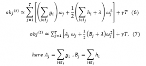
It was used for further enhancement by hyperparameter tuning of n_estimator. n_estimator hyperparameter in XGboost is cunt of trees to fit. It is also number epochs the algorithm is run to add a tree until the number of trees reaches n_estimator count to further improve the accuracy[14,36] of the model. The default value of n_estimators is 100. For group 4, Figure 3 shows classification error, Figure 4 shows area under the curve for n_estimator =100 and Figure 5 log loss with n_estimator=100. It shows that the model is not overfitting and has room for improvement. Hence, further hyperparameter tuning is done for group4, selectionset#4, with n_estimators = 200, 300, and thereafter with 400.

Table 5: Comparison of Prediction Efficiency for Regrouped Data

Sl no.	Name of datasets	Accuracy	AUC
1	Raw byte histogram	93.28%	.978743
2	Byte Entropy	90.69%	.967944
3	Strings	92.2845%	.97618
4	Strings, General, Optional Header, Sections	95.4405%	.992099
5	Imports of API with DLL	92.05%	.977229
6	Exports of API	58.8985	.597902
7	Base dataset with LightGBM[1]	98.162%	.999112
8	With All features as in Base dataset	97.09	.99571

Table 6: Group 4 Performance Parameter

Sl n.	n_estimator	Accuracy	AUC	logloss	Classification error
1	200	96.537%	.995015	.10523	.03462
2	300	97.07%	.996472	.08768	.02713
3	400	97.49%	.997261	.07675	.02445

Table6: COMPARISON OF PREDICTION EFFICIENCY FOR REGROUPED DATA   Sl no. Name of datasets Accuracy AUC 1 Raw byte histogram 93.28% .978743 2 Byte Entropy 90.69% .967944 3 Strings 92.2845% .97618 4 Strings, General, Optional Header, Sections 95.4405% .992099 5 Imports of API with DLL 92.05% .977229 6 Exports of API 58.8985 .597902 7 Base dataset with LightGBM[1] 98.162% .999112 8 With All features as in Base dataset 97.09 .99571

Table 6 shows the improvement in performance parameters for accuracy, AUC, and logloss. The accuracy and AUC for group4 with merely 431 features are comparable to the performance of the base dataset with 2351features. Figure 6 shows classification error, Figure 7 shows AUC, and Figure 8 shows log loss for n_estimator=400. Table 6 shows the accuracy and AUC for n_estimator 200, 300, 400. The accuracy for just 431 features is 97.495 higher than the accuracy with all the 2351 features 97.09 % using XGBoost with n_estimator = 400. Further feature selection has been done that matches the performance of the base dataset or improves in some performance parameters for classification.

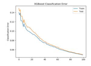
Figure 3: XGBoost classification Error  for n_estimator = 100

Figure 4: XGBoost AUC for n_estimator = 100

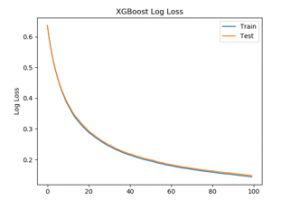
Figure 5: XGBoost Logloss for n_estimator = 100

Results Experiment part3

Inclusion or exclusion of features representing more than one MZ had no effects on prediction efficiency. On further investigation using the SHA-256 signature at virustotal [3], it was found that benign application may package up to 32 executable for software upgrade purposes

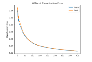
Figure 6: XGBoost classification Error for n_estimator = 400

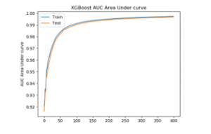
Figure 7: XGBoost AUC for n_estimator = 400

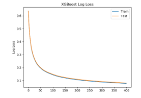
Figure 8: XGBoost logloss for n_estimator = 400

Results Experiment part4

A model was built with these selected 276 features and prediction efficiency were explored. The accuracy, AUC, and logloss parameters for the n_estimators  600 are tabulated in Table 5 and compared with base datasets. The accuracy has given a 1% increase compared with only subset#4  in Table 7. It has exceeded the accuracy of all the features in the base dataset by 1.41% (98.5% vs 97.09%). It has also exceeded the accuracy compared to the base set at 98.2% as reported by author in [5]. The AUC value is marginally less .999112 vs .99872.

Figure 9:Feature importance selected 276 features, number times called

Table 7: Accuracy, Auc for Base Dataset and 276 Features as Per Feature Importance

Sl no.	n_estimator	Accuracy	AUC	logloss	Classification error
1	Base dataset [1] using LightGBM	98.162%	.999112	NA	NA
2	With All features as in Base dataset	97.09	.99571	NA	NA
3	Select 276 feature sets, n_estimator=600	98.5%	.998972	.046314	.014157
4	Group4 feature sets, n_estimator=600	97.49%	.997261	.076753	.024453

5.4. Further reduction in important features

The feature importance of these selected 276 is further studied. It was found that all the selected features contributed to building the classifier model. Unlike with base dataset, in which there were 2075 features were noisy and did not contribute to building the model. None of the selected 276 falls into the category which does not contribute to building the model using XGboost.

Figure 9 gives how many times a feature is used for generating the GDBT model using the XGboost method. The actual figure is not legible due to the 276 feature. Hence, the only top part of the results of the feature is shown in each figure.

5.5. Hyperparameter tuning with learning rate

We tried to optimize the model with a change in the learning rate. The default learning rate in XGBoost is 0.1. We tried with a learning rate of 0.01 and n_estimator=600. The model build gave slow movement to performance parameters as in the default learning rate. We used learning rate of 0.15 and .2 with n_estimators = 600. It indicates that the model gives the same efficiency but at a different rate. Hence, performance parameters are not affected at n_estimator = 600 for various learning rates.  There was no improvement in performance parameters.

Table 8: Performance of XGBoost with other classification algorithm

Models	Accuracy (%)	Precision	Recall	F-score	Time in Second
Gaussian Naïve Bayes	51.82	0.43	0.10	0.17	470.37
KNN	56.38	0.52	0.88	0.65	307.66
Linear SVC	49.98	0.48	0.99	0.65	115.62
Decision Tree	89.62	0.85	0.94	0.89	177.43
AdaBoost	89.24	0.87	0.91	0.89	105.06
Random Forest	93.6	0.9	0.98	0.93	141.54
ExtraTrees	94.68	0.92	0.98	0.94	47.62
GradientBoosting	93.16	0.89	0.98	0.93	72.83
XGBoost	93.04	0.89	0.98	0.93	106.89
XGB with trained model  1	97.72	0.98	0.97	0.98	63.24
XGB with trained model  2	98.22	0.99	0.98	0.98	61.44

5.6. Comparison with other classification algorithm

Eight other classification algorithms were compared with the XGBoost classification algorithm on a sub dataset of 5000K Training and 5000k test datasets with selected 276 features. The performance of these algorithms is listed in table 8. XGBoost indicates classification performance without hyperparameter tuning, XGB with trained model 1 is the tuned model with n_estimator = 400 and XGB with trained model 2 is the tuned model with n_estimator = 600. It indicated the performance score of XGB with trained model 2 is best among all the classification algorithm. XGBoost is better than Gaussian naïve Bayes, K-Nearest Neighbour (KNN), Linear SVC, Random forest, and Decision tree in terms of the time to make model and test for sub dataset. Extratrees, GradientBoosting, Adaboosts are better than XGBoost in terms of time to train and test the model for the identified sub dataset.

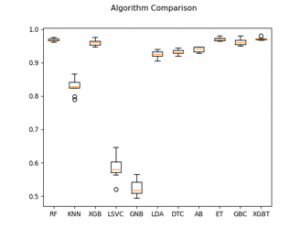
Figure 10: Algorithm comparison with Accuracy with 10-fold cross validation

5.7. K-fold Cross-validation of algorithms

Cross-validation is a statistical method to validate the classification algorithm. 10 fold cross-validation was done with the same sub data set as above with 5000 K training data set with selected 276 features and eight different classification algorithms. Figure 6 displays a whisker and box plot for the accuracy of eight different classification algorithms and a trained XGBoost model. The XGBT is the label for the trained XGBoost model. The cross-validation for the model makes the smallest box in the Figure 10. It means the model does not have much variation for the accuracy while performing the 10 fold cross-validation. It indicates the model is optimized well with hyperparameter tuning.

5.8. Comparison with other works

Table 9 compares the result of this research with other similar work, identified with reference in the column, which have used either the dataset given in [5] in part or full or other very large datasets for building malware classifier. The accuracy is marginally low compared to [48] as they have used 1/3 of the samples. It is also low compared to author using deep convolution malware classifier in [49, 50]. They have used high-end computing resources with 1711 features. In [50] author saves computation time by detecting malware during the static analysis and prevent dynamic analysis of malware in the Security Operation Center. Such work to use the large dataset with low-end computing is not available at this time and is one of the contributions. We have achieved higher accuracy using low computing resource of intel i5 processor and reduced 276 number of features compared other works which use high-end computing.

Table 9: Comparison with Other Works

	Robust intelligent MWD using DL[48]	Ember [5]	Malconv[11]	The Need for speed, Brazillian MWC[26]	DEEP CONVOLUTIONAL MALWARE CLASSIFIERS [49]	Static PE Malware Detection[50]	XGBoost	A hybrid static tool for dynamic detection of MW [51]
Size of Data	70148 Benign, 69860 malware Static Analysis part	800K	2 Million	21116 Benign 29704 Malware	20 Million	800K	800K	195,255 Benign, 223,352 malware
Results – Accuracy	98.9 highest by DNN	98.2	92.2	98	97.1	99.394	98.5	98.73%
AUC	Not Specified	0.99911	0.99821	Not Specified	76.1 for  interval 0-.001	0.999678	0.998972	Not Specified
Processor Used	Intel Xeon	Intel i7	Not Specified	Not Specified	Not Specified	24 v CPU Google Compute Engine	Intel i5	Not Specified
No of features	Not Specified	2351	not applicable	25 PE header + 2 hash	538, 192	1711	2351, (276)	4002 features from static analysis. 4594 features from dynamic analysis
GPU	Yes,	NO	8 x DGX-1	Not Specified	Not specified	NO	NO	Not specified
Train Data	42140 Benign 41860 Malware	300K Benign 300K Malware	2 Million	.5×21116 Benign .5×29704 Malware	20 Million	300K Benign 300K Malware	300K Benign 300K Malware	Not specified
Time	Not available	20 Hours	25 hours /Epoch 250 Hours	Not available	Not available	5 minutes	1315 seconds without hyper parameter tunning	Not specified

6. Conclusion

Dataset had been regrouped into various groups with domain expertise in malware detection to build efficient models with low computational resources without GPUs. The regrouped data with strings extraction, general, header, section with just 431 feature sets compared to 2351 gives comparable efficiency in prediction performance at n_estimator=400. The model is further improved considering the feature importance as given by XGBoost and selected 276 features from 2351 features in base original data. Selected features are used to generate models using XGboost, with low-end computing resources compared to other similar work. The model with the selected feature gives improved prediction performance. The features learned can be widely useful if the performance parameters are the same across datasets. All the hashed feature derived from the export function group did not contribute to build an efficient model and to predict the malware.

Although the open base dataset is very large and balanced, the malware in datasets may not be exporting the API Calls or private APIs for malware activities. Hence, the export part of the features of the dataset did not contribute to building the model. However, this may not be always true. Shared biases are minimized if the data is from different sources. The sources of data for base datasets are not known. It also gives an upper and lower bound of accuracy.

Ember dataset is for windows executable. Using LIEF methodology in [12], we can generate datasets for other operating systems such as Linux, Mac os Android, etc. The challenge remains to get the malware samples for other OS. The techniques described here can be used to generate a model using low computational resources that can predict malware efficiently. Further, the study may be possible to determine which exact features from the PE format of application or file agnostic features are part of the selected feature.

To our knowledge, this research is one of its kind that uses a full dataset with the XGBoost GBDT algorithm to get matching or higher accuracy with a low computing resource. The basic model using the XGBoost classification algorithm was trained using low computation resources in 1315 seconds with a reduction in the feature set. The hyperparameter tuned model gives improved performance for accuracy of 98.5 and on par  AUC of .9989.

Conflict of Interest

The authors declare no conflict of interest.

1. V. Blue, RSA: Brazil’s “Boleto Malware” stole nearly $4 billion in two years, https://www.zdnet.com/article/rsa-brazils-boleto-m.
2. F. Cohen, “Theory and Experiments,” 6, 22–35, 1987. https://doi.org/10.1016/0167-4048(87)90122-2
3. https://www.virustotal.com
4. C. Rossow, C.J. Dietrich, C. Grier, C. Kreibich, V. Paxson, N. Pohlmann, H. Bos, M. Van Steen, “Prudent practices for designing malware experiments: Status quo and outlook,” Proceedings – IEEE Symposium on Security and Privacy, (June 2014), 65–79, 2012, doi:10.1109/SP.2012.14.
5. H.S. Anderson, P. Roth, “EMBER: An Open Dataset for Training Static PE Malware Machine Learning Models,” 2018. https://arxiv.org/abs/1804.04637
6. M. Pietrek, Inside windows-an in-depth look into the win32 portable executable file format, MSDN Magazine, 2002. https://docs.microsoft.com/en-us/previous-versions/bb985992(v=msdn.10)?redirectedfrom=MSDN
7. D. Devi, S. Nandi, “PE File Features in Detection of Packed Executables,” International Journal of Computer Theory and Engineering, (January), 476–478, 2012, doi:10.7763/ijcte.2012.v4.512.
8. D. Baysa, R.M. Low, M. Stamp, “Structural entropy and metamorphic malware,” Journal in Computer Virology, 9(4), 179–192, 2013, doi:10.1007/s11416-013-0185-4.
9. M. Sebastián, R. Rivera, P. Kotzias, J. Caballero, Avclass: A tool for massive malware labeling, 230–253, 2016, doi:10.1007/978-3-319-45719-2_11.
10. E. Raff, R. Zak, R. Cox, J. Sylvester, P. Yacci, R. Ward, A. Tracy, M. McLean, C. Nicholas, “An investigation of byte n-gram features for malware classification,” Journal of Computer Virology and Hacking Techniques, 14(1), 2018, doi:10.1007/s11416-016-0283-1.
11. E. Raff, J. Barker, J. Sylvester, R. Brandon, B. Catanzaro, C. Nicholas, “Malware Detection by Eating a Whole EXE,” 2017, doi:10.13016/m2rt7w-bkok.
12. Quarkslab, LIEF: library for instrumenting executable files, https://lief.quarkslab.com/.
13. M.Z. Shafiq, S.M. Tabish, F. Mirza, M. Farooq, “PE-miner: Mining structural information to detect malicious executables in realtime,” Lecture Notes in Computer Science (Including Subseries Lecture Notes in Artificial Intelligence and Lecture Notes in Bioinformatics), 5758 LNCS, 121–141, 2009, doi:10.1007/978-3-642-04342-0_7.
14. A. Moser, C. Kruegel, E. Kirda, “Limits of static analysis for malware detection,” Proceedings – Annual Computer Security Applications Conference, ACSAC, 421–430, 2007, doi:10.1109/ACSAC.2007.21.
15. M.Z. Shafiq, S.M. Tabish, F. Mirza, M. Farooq, “PE-miner: Mining structural information to detect malicious executables in realtime,” Lecture Notes in Computer Science (Including Subseries Lecture Notes in Artificial Intelligence and Lecture Notes in Bioinformatics), 5758 LNCS, 121–141, 2009, doi:10.1007/978-3-642-04342-0_7.
16. F. Guo, P. Ferrie, T.C. Chiueh, “A study of the packer problem and its solutions,” Lecture Notes in Computer Science (Including Subseries Lecture Notes in Artificial Intelligence and Lecture Notes in Bioinformatics), 5230 LNCS, 98–115, 2008, doi:10.1007/978-3-540-87403-4_6.
17. M.G. Schultz, E. Eskin, E. Zadok, S.J. Stolfo, “Data mining methods for detection of new malicious executables,” Proceedings of the IEEE Computer Society Symposium on Research in Security and Privacy, (February 2001), 38–49, 2001, doi:10.1109/secpri.2001.924286.
18. M. Alazab, S. Venkataraman, P. Watters, “Towards understanding malware behaviour by the extraction of API calls,” Proceedings – 2nd Cybercrime and Trustworthy Computing Workshop, CTC 2010, (July 2009), 52–59, 2010, doi:10.1109/CTC.2010.8.
19. M. Egele, T. Scholte, E. Kirda, C. Kruegel, “A survey on automated dynamic malware-analysis techniques and tools,” ACM Computing Surveys, 44(2), 2012, doi:10.1145/2089125.2089126.
20. M. Carpenter, T. Liston, E. Skoudis, “Hiding virtualization from attackers and malware,” IEEE Security and Privacy, 5(3), 62–65, 2007, doi:10.1109/MSP.2007.63.
21. T. Raffetseder, C. Kruegel, E. Kirda, “Detecting system emulators,” Lecture Notes in Computer Science (Including Subseries Lecture Notes in Artificial Intelligence and Lecture Notes in Bioinformatics), 4779 LNCS, 1–18, 2007, doi:10.1007/978-3-540-75496-1_1.
22. R. Pascanu, J.W. Stokes, H. Sanossian, M. Marinescu, A. Thomas, “Malware classification with recurrent networks,” ICASSP, IEEE International Conference on Acoustics, Speech and Signal Processing – Proceedings, 2015-August, 1916–1920, 2015, doi:10.1109/ICASSP.2015.7178304.
23. J. Saxe, K. Berlin, “Deep neural network based malware detection using two dimensional binary program features,” 2015 10th International Conference on Malicious and Unwanted Software, MALWARE 2015, 11–20, 2016, doi:10.1109/MALWARE.2015.7413680.
24. W. Huang, J.W. Stokes, “MtNet: A multi-task neural network for dynamic malware classification,” Lecture Notes in Computer Science (Including Subseries Lecture Notes in Artificial Intelligence and Lecture Notes in Bioinformatics), 9721, 399–418, 2016, doi:10.1007/978-3-319-40667-1_20.
25. B. Kolosnjaji, A. Zarras, G. Webster, C. Eckert, “Deep learning for classification of malware system call sequences,” Lecture Notes in Computer Science (Including Subseries Lecture Notes in Artificial Intelligence and Lecture Notes in Bioinformatics), 9992 LNAI, 137–149, 2016, doi:10.1007/978-3-319-50127-7_11.
26. F. Ceschin, F. Pinage, M. Castilho, D. Menotti, L.S. Oliveira, A. Gregio, “The Need for Speed: An Analysis of Brazilian Malware Classifers,” IEEE Security and Privacy, 16(6), 31–41, 2019, doi:10.1109/MSEC.2018.2875369.
27. R. Ronen, M. Radu, C. Feuerstein, E. Yom-Tov, M. Ahmadi, “Microsoft Malware Classification Challenge,” http://arxiv.org/abs/1802.10135, 2018.
28. J. Jang, D. Brumley, S. Venkataraman, “BitShred: Feature hashing malware for scalable triage and semantic analysis,” Proceedings of the ACM Conference on Computer and Communications Security, 309–320, 2011, doi:10.1145/2046707.2046742.
29. J.Z. Kolter, M.A. Maloof, “Learning to detect malicious executables in the wild,” KDD-2004 – Proceedings of the Tenth ACM SIGKDD International Conference on Knowledge Discovery and Data Mining, 7, 470–478, 2004, doi:10.1145/1014052.1014105.
30. K. Weinberger, A. Dasgupta, J. Langford, A. Smola, J. Attenberg, “Feature hashing for large scale multitask learning,” ACM International Conference Proceeding Series, 382, 2009, doi:10.1145/1553374.1553516.
31. Jason Brownlee, XGBoost with Python Gradient Boosted Trees with XGBoost and sci-kit learn. Edition: v1.10
32. https://xgboost.readthedocs.io/en/latest/python/python_api.html
33. https://lightgbm.readthedocs.io/en/latest/Python-Intro.html
34. Ke, G., “LightGBM: a highly efficient gradient boosting decision tree.” In: Advances in Neural Information Processing Systems, pp. 3149–3157 (2017). http://papers.nips.cc/paper/6907-lightgbm-a-highly-efficient-gradient-boosting-decision-tree
35. K. Raman, “Selecting Features to Classify Malware,” InfoSec Southwest 2012, 1–5, 2012.
36. A.H. Sung, J. Xu, P. Chavez, S. Mukkamala, “Static Analyzer of Vicious Executables (SAVE),” Proceedings – Annual Computer Security Applications Conference, ACSAC, (January), 326–334, 2004, doi:10.1109/CSAC.2004.37.
37. H. Daku, P. Zavarsky, Y. Malik, “Behavioral-Based Classification and Identification of Ransomware Variants Using Machine Learning,” Proceedings – 17th IEEE International Conference on Trust, Security and Privacy in Computing and Communications and 12th IEEE International Conference on Big Data Science and Engineering, Trustcom/BigDataSE 2018, 1560–1564, 2018, doi:10.1109/TrustCom/BigDataSE.2018.00224.
38. A. Damodaran, F. Di Troia, C.A. Visaggio, T.H. Austin, M. Stamp, “A comparison of static, dynamic, and hybrid analysis for malware detection,” Journal of Computer Virology and Hacking Techniques, 13(1), 2017, doi:10.1007/s11416-015-0261-z.
39. M. Tang, Q. Qian, “Dynamic API call sequence visualisation for malware classification,” IET Information Security, 13(4), 367–377, 2019, doi:10.1049/iet-ifs.2018.5268.
40. L. Nataraj, D. Kirat, B. Manjunath, G. Vigna, “SARVAM: Search And RetrieVAl of Malware,” Ngmad, (January), 2013.
41. L. Nataraj, S. Karthikeyan, G. Jacob, B.S. Manjunath, “Malware images: Visualization and automatic classification,” ACM International Conference Proceeding Series, 2011, doi:10.1145/2016904.2016908.
42. D. Kirat, L. Nataraj, G. Vigna, B.S. Manjunath, “SigMal: A static signal processing based malware triage,” ACM International Conference Proceeding Series, (March 2016), 89–98, 2013, doi:10.1145/2523649.2523682.
43. S. Geetha, N. Ishwarya, N. Kamaraj, “Evolving decision tree rule based system for audio stego anomalies detection based on Hausdorff distance statistics,” Information Sciences, 180(13), 2540–2559, 2010, doi:10.1016/j.ins.2010.02.024..
44. S. Venkatraman, M. Alazab, “Use of Data Visualisation for Zero-Day Malware Detection,” Security and Communication Networks, 2018, 2018, doi:10.1155/2018/1728303..
45. A.P. Bradley, “The use of the area under the ROC curve in the evaluation of machine learning algorithms,” Pattern Recognition, 30(7), 1145–1159, 1997, doi:10.1016/S0031-3203(96)00142-2.
46. T. Chen, Introduction to Boosted Trees.. http://homes.cs.washington.edu/~tqchen/pdf/BoostedTree.pdf
47. E. Raff, J. Sylvester, C. Nicholas, “Learning the PE header, malware detection with minimal domain knowledge,” AISec 2017 – Proceedings of the 10th ACM Workshop on Artificial Intelligence and Security, Co-Located with CCS 2017, 121–132, 2017, doi:10.1145/3128572.3140442.
48. R. Vinayakumar, M. Alazab, K.P. Soman, P. Poornachandran, S. Venkatraman, “Robust Intelligent Malware Detection Using Deep Learning,” IEEE Access, 7, 46717–46738, 2019, doi:10.1109/ACCESS.2019.2906934.
49. M. Krčál, O. Švec, O. Jašek, M. Bálek, “Deep convolutional malware classifiers can learn from raw executables and labels only,” 6th International Conference on Learning Representations, ICLR 2018 – Workshop Track Proceedings, (2016), 2016–2019, 2018.
50. H. Pham, T.D. Le, T.N. Vu, Static PE Malware Detection Using Gradient, Springer International Publishing, 2018, doi:10.1007/978-3-030-03192-3.
51. D. Kim, D. Mirsky, A. Majlesi-Kupaei, R. Barua, “A Hybrid Static Tool to Increase the Usability and Scalability of Dynamic Detection of Malware,” MALWARE 2018 – Proceedings of the 2018 13th International Conference on Malicious and Unwanted Software, 115–123, 2019, doi:10.1109/MALWARE.2018.8659373.

(Click Here)

(Click Here)