1. Introduction

The advancement in clinical and healthcare practice today is due to the vast database explosion. Hospitals, health professionals, and treatment centers disclose medical data to the community to call for mutual support and benefit. The data availability is expanding in many forms, both the number of known attributes and the number of new observations [2]. We can see an excellent example from the widely published new coronavirus (COVID-19) data [3]. However, due to privacy concerns, medical data is abundant, but it is also very sparse, which we only have on specific individuals. A country’s medical data may not be relevant to develop solutions for the same disease in another country. That creates challenges and difficulties for traditional medical diagnosis because many observations are lost due to a lack of information. The central issue is that health data is characterized by the considerable complexity of detecting culty, medical data exists in many different structures. For example, numbers, categories, text, images, and time-series make medical diagnosis even more difficult. However, from the benefit of big data to health care, leveraging medical data collection offers an excellent opportunity to improve the efficiency of healthcare provider [4, 5]. Current challenges in health practice include information overload, confounding attributes, and noise data in different populations, making manual analysis of experts ultimately difficult [6, 7]. The cost of using medical professionals to examine multiple clinical cases accumulated over time is very high. From a medical diagnosis, one can argue that there is an urgent need to work with a wide variety of data, leverage useful knowledge, and recommend a system that can make the most of information from that data.

Classification is an essential task in health diagnostic systems.

We use observed metrics to classify samples into different diseases, or separate degrees of the same illness [8, 9]. Clinicians are trained and have the solid knowledge to classify diseases based on sample data accurately. We can agree that correctly distinguish the right disease is one of the fundamental bases for effective treatment of the disease. However, as more data appears in clinical fields, the existing manual diagnostic process that relies on expert expertise cannot be applied quickly and effectively. As a result, the course of treatment may have to be done more slowly or eliminated. Addressing mentioned problems lies in the interactions between healthcare and automation decisions based on machine learning, applying to the classification problem. Thus, one can argue that the classification design is an iterative process between machine learning and available clinical sources to demonstrate the implications of a medical diagnostic procedure. Consequently, the authors turn our attention to proposing processes that automatically select the most suitable machine learning models for each of the different types of data as the foundation of building and recommending diagnostic procedures.

The classic definition of machine learning is ”A computer program is said to learn from experience E with respect to some class of tasks T and performance measure P, if its performance at tasks in T, as measured by P, improves with experience E”. It was initially described as a computer program that learns to automatically perform a required task or make a decision from data without explicitly programmed. This definition is comprehensive and can cover almost any set of data-driven approaches. Machine learning has been dramatically advanced over several decades, from theory context to a general business and technology implementation. Especially in healthcare research, it is obvious to perceive the scrutinizing implementation of machine learning to warranty the rewarded benefits in early disease detection, service recommendation, and patientoriented information offering [10]–[13]. There are two substantially interrelated questions in medical diagnosis: How can computer scientists build machine learning programs that automatically improve through experience, e.g., through data? How can practitioners and clinical experts incorporate with these machine learning programs? The first question can be addressed by marriage between machine learning models and vast medical data. The more data we feed into the learning algorithms, the more accurate the prediction is. Whatever the machine learning models are used, the fundamental expectation is to generalize the knowledge from training data to unseen observations. It is the generalization capacities of learning approaches on how robust they are to their modeling assumptions or the errors in the test set. However, many practitioners and researchers have eventually recognized that there is no absolute winner approach to all kinds of data. The reasons can be broken down into many considerations. The prediction accuracy is diminished when the quantity and quality of clinical data are incomplete.

Different regions expose unique characteristics of a particular disease, which may affect the generalization capacities of learning models [13]. The privacy of medical records also subtracts the high availability of data for research. It is inadvertently possible that racial biases might be built into healthcare systems [14]. The reason might be placed at the characteristics of machine learning models themselves. Even when implicit, the learning approaches generally reply to learn parameters, hyperparameters tuning to find the best values for these coefficients that optimize a particular evaluation metric. Consequently, the use of machine learning is complicated and should not rely on one single model since the correct diagnosis in a particular circumstance can be controversial. Hence, an effective workflow should effortlessly incorporate a diversity of learning models and select the best candidate for a particular input data. It comes to the design idea of black-box models [15] in unintended consequences of machine learning in medicine. The workflow should work with various types of input data and transparently amalgam

ate diverse models. In that setting, different learning approaches for medical diagnosis are evaluated to select the most accurate one. More importantly, the result’s interface should also be attractive to enhance hospital experts and end-users’ incorporation.

Today, smartphones are one of the most ubiquitous communication devices and the fastest growing technology industry sectors. An increasing number of mobile applications have been developed to perform a comprehensive spectrum of daily tasks and entertainment. Its impact on medical treatment has already been significant on a global scale. In this paper, the authors deploy an Android mobile application to illustrate how the proposed workflow integrates with hospital experts and patients as end-users. Mobile health is a new concept that describes services supported by mobile communication devices such as smartphones, tablets, smartwatches, patient monitoring devices. However, the discussion of mobile health is out of our research scope. Interesting readers might refer to several mindful papers in the literature [16]–[18].

To be the best of our knowledge, the authors have made several contributions as follows:

• We sharp the connection between the automatic selection of machine learning models for classification in medical diagnosis.
• We extend the pool of machine learning models, including a single approach, bagging algorithm, and advanced boosting technique. We prove that there is no winner model to address medical data sources.
• We extend the background of machine learning algorithms in much more details.
• We extend the experiments section where we carefully describe experimental results, reproducibility, and mobile app development.

The rest of the paper is organized as follows. Section 2 gives a general idea of how our proposed workflow works and how the best learning model is selected. Then in Section 3, the authors introduce required machine learning materials and methodology that need to comprehend the experiments. More specifically, we discuss several well-known machine learning models and evaluation metrics. Our intensive comparison is then discussed in Section 4 in which we go through data collection, experimental results, reproducibility, and mobile app development. Finally, several final thoughts are presented in Section 5.

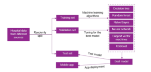
Figure 1: Automatic Selection of Machine Learning Models.

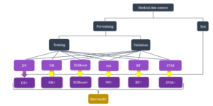
Figure 2: Hyperparameters tuning for picking the most appropriate learning approach.

2. Interpretation of Machine Learning the validation set. Finally, the instances that are considered as un-

Models seen data belong to the test dataset. Figure (3) illustrates a practical splitting protocol in machine learning. This selection mechanism is described in Figure (2). The authors apply decision trees (DT), na¨ıve

As mentioned in the previous discussion, the authors propose pro-

Bayes (NB), artificial neural networks (NN), random forest (RF), cesses that interpret the most appropriate learning models for each support vector machines (SVM), and extreme gradient boosting of the different clinical datasets as the foundation of developing and

(XGBoost). recommending diagnostic procedures. The whole process works as (i) hyperparameters tuning for picking the most appropriate learning approach, and (ii) a mobile application is developed to support clinical practices, see Figure 1. Here, clinical experts might not need to understand the technical part because it is done automatically. Experts feed hospital data from different sources to the system. First, data preparation starts with splitting sources into training-validationtest schemes. The training and validation sets are feed into a black box of several predefined learning models. The best model is selected based on an evaluation metric’s optimization, performing on ^{Figure 3: A visualization of the dataset splitting.}

3. Materials and Methodology

In this section, the authors briefly present the implemented machine learning approaches. We do not pretend that our discussion will be an overview of models. Interesting readers might refer to several textbooks for further self-learning and comprehension [19]–[22]. Furthermore, other interesting papers that connect the gap between machine learning and medical research can be found at [23]–[26].

3.1. Support Vector Machines

SVM constructs a hyperplane in a high dimensional space. Assuming that the linear model is v^T x, then the following constraints need to be satisfied in case of the data points are linearly separable:

SVM seeks to find a good hyperplane where the margin to different classes’ data points is maximum. Hence, SVM optimizes:

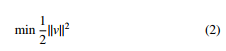
In case of non-linear separation, the constraints cannot be fulfilled. Then, soft margin is applied. The optimization in Equation 2 becomes

minkvk² + C ^Xσ_i,

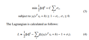
Setting the respective derivatives to 0, then the dual form of the optimization is as follows:

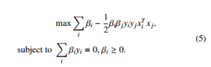
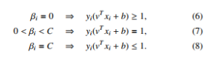
where the ranking model v = ^P_i α_iy_ix_i is achieved by solving the quadratic programming. The optimality in Equation 5 is applied by the Karush-Kuhn-Tucker (KTT) conditions. Then we get:

3.2. Na¨ıve Bayes

Due to its easy implementation and high performance, many machine learning practitioners consider Na¨ıve Bayes is a simple but effective machine learning model [27]. We denote a vector x, a set τ and y = s as model’s parameters and accompanying label respectively. Then, we can define a generative model x as follows:

P(y = s|x,τ) = _P s0 P(y = s0|τ)P(x|y = s0,τ) , (9) where P(x|y = s,τ), P(y = s|x) are class-conditional density and class posterior. P(y = s) is class prior. Equation (9) can be proportionally calculated as follows:

Then, the class-conditional density in Equation (9) is estimated as follows:

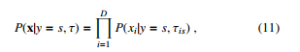
which is the Na¨ıve Bayes classifier. Because it is not expected that the features should be independent, Equation (11) can be re-written depending on each feature’s type, e.g. binary, real-valued, or categorical attributes. Specifically, in case of binary attributes, the Bernoulli distribution can be utilized as follows:

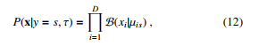
where µ_is means the probability of attribute i objected to class s. In case of real-valued attributes, the Gaussian distribution can be computed as follows:

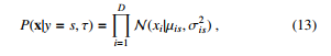
where µ_is and σ²_is mean the probability of attribute i objected to class s and its variance respectively. In case of categorical attributes, multinoulli distribution is used as follows:

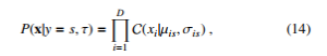
where x_i ∈ {1,…, K} is categorical attributes and σ_is is a histogram over K.

In our research, disease classification is basically to classify input vector into different categories. Depending on the representation as a binary or real-valued matrices, Equation (12 or 13) is applied to make prediction.

3.3. Artificial Neural Networks

We apply Multilayer Perceptrons as the version of artificial neural networks applied in the experiments. We form the the model as follows:

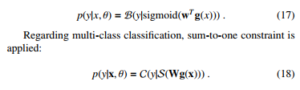
where H is the number of hidden units, f is a logical function. V is the weight matrix from the inputs to the hidden nodes, while w is the weight vector from the hidden nodes to the output. In our experiments, we deploy an artificial neural network with 2 hidden layers due to the hardware constraints. A sigmoid function is activated on the output if the classification is binary.

3.4. Decision Trees

We denote R as the number of regions, w_r is the weight response in the r region. A decision tree is formed as follows.

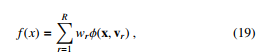
where v_r is the choice of variable to split on.

To find the best partitioning of the input data, the greedy procedure is used in common. There is progress that measures the quality of a split in the classification setting. Given a threshold t, we fit a multinoulli model to the data that satisfies the condition X_j < t by estimating the class-conditional probabilities as follows:

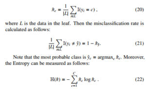
We leave the Entropy as the default setting for the decision tree in our experiments.

3.5. Bagging Aggregation with Random Forest

Although DT is one of the most effective and speedy models, it is highly variable due the the splitting. At first, DT is trained on a complete dataset. Then that dataset is split into two portions. DT is applied on the two portions and interestingly, they return different results. The idea of bagging technique helps to reduce the variance in any model [28]. An example of bagging is the generation of many decision trees in parallel. We can train T different trees on different subsets of the data, chosen randomly with replacement, and then compute the ensemble as follows:

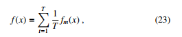
where f_t is the t’th tree. This helps reduce the variance of the predictions.

3.6. Boosting Technique with XGBoost

XGBoost, see Figure 4, is a popular and efficient machine learning implementation of the gradient boosted trees [29]. It has been widely applied in some data competitions. The general idea of gradient boosting is to predict a class by combining several weak learners. XGBoost used a regularized objective function (L1 and L2) that combines a convex loss function (emerging from the difference between the ground-truth and prediction) and a penalty term for controlling model complexity. A gradient descent algorithm is used to minimize the loss when adding new learners. The training proceeds iteratively, adding new trees that predict the prior trees’ residuals associated with previous trees to perform the final prediction. Regularization is included to reduce overfitting. The authors denote the i-th instance with an associated label as x_i ∈ R^d, yˆ as the prediction given x_i. T is the number of trees. Then we define:

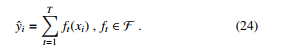
Machine learning is basically the procedure of learning parameters θ = {w_j| j = 1,…,d}. The objective function is follows:

where L(θ) is the training loss and Ω(θ) is the regularization configuration. Optimizing L(θ) results in high prediction accuracy, while optimizing Ω(θ) balances the simplicity of model. For each iteration j, we define the XGBoost objective function by expanding Equation

(25).

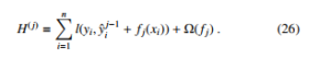
We can see that we cannot optimize Equation (26) by using traditional optimization methods because XGBoost objective is a function of functions. However, we can transform the original objective function to the Euclidean domain by Taylor approximation [30].

The first order gradient statistics is defined as g_i = ∂_yˆt₋₁l(y_i,yˆ^t−1), while the second order gradient statistics of the loss function is defined as h_i = ∂²_yˆt₋₁l(y_i,yˆ^t−1):. Hence, Equation (26) can be rewritten as follows:

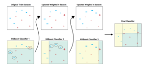
Figure 4: The sequential ensemble methods in XGBoost.

4. Experiments

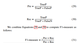
4.1. Evaluation Metrics: F1-measure

We denote TrueP, FalseP, and FalseN as true positive, false positive, and false negative. With the classification problem where the classes’ data sets are very different from each other, there is a logical operation commonly used as Precision-Recall. First of all, consider the problem of binary classification. We also consider one of the two classes to be positive and the other to be negative. With a way of determining a class to be positive, precision (Pre) is defined as the ratio of the number of true positive points to those classified as positive (TrueP + FalseP). The recall (Rec) is defined as the ratio of the number of true positive points to positive (TrueP + FalseN). Mathematically, Precision and Recall are two fractions with equal numerators but different denominators:

4.2. Dataset Collection

In this paper, eight datasets related to medical data are selected from the UCI Machine Learning Repository. More specifically, the experimental datasets are Breast Cancer Data^[1], Heart Disease Data^[2], Dermatology Data^[3], Vertebrae Data^[4], Hepatitis Data^[5], Cervical cancer (Risk Factors) (RF) Data^[6], Autism Adolescent Data^[7], and Diabetes Data^[8]. The authors prudentially select several categorization datasets that are suitable for the research’s scope. Categorical attributes are converted into numerical representation using a onehot encoding process. Data imbalance is accepted as the native characteristics of classification data sources. The eight experimental datasets are shown in Table (1).

Table 1: Hospital data from different sources

#	Dataset	Prediction Type	# Samples	# Attributes
1	Breast Cancer	Binary	286	9
2	Dermatology	Multi class	365	22
3	Heart Disease	Multi class	303	13
4	Hepatitis	Binary	155	19
5	Vertebrae	Multi class	310	6
6	Cervical Cancer (RF)	Binary	858	32
7	Autism Adolescent	Binary	768	20
8	Diabetes	Binary	104	8

In the experiments, the authors set up the splitting scheme by the following ratios. First, we randomly split without replacement the dataset into 70% and 30% for the pre-training and test parts respectively. Next, the pre-training portion is randomly split without replacement into 80% and 20% for the training and validation portions respectively. The role of these sets is introduced above, see Figure (2).

4.3. Experimental Results

As mentioned above, the model’s performance is judged by its ability to predict unseen data accurately. Hence, the best scores are considered on the test sets. The F1-measure of experimental models performing on datasets are summarized in Table (2). Overall, there is no absolute best approach. However, the random forest model achieves remarkable performance on four different datasets, e.g., Breast Cancer, Cervical Cancer, Autism, and Diabetes. The neural network approach gets the least performance since it does not win any best prediction.

One interesting point to note is that Na¨ıve Bayes algorithm achieves the F1-measure of 1.0 on the Dermatology data. Meanwhile, XGBoost gains the F1-measure of 0.94 on the Diabetes dataset. RF is the best models performing on four different data, namely Breast Cancer, Hepatitis, Cervical Cancer (RF), and Autism Adolescent. Observing all experimental datasets, Vertebrae is the most challenging. Even the best model, e.g., SVM, only achieves the F1-measure of 0.54. Statistics in Table (1) show that Cervical Cancer has the most instances and the most attributes, e.g., 858 and 32, respectively. Even though Cervical Cancer has the most observations, one can argue that only partial representations of properties might not be enough to learn coefficients for 32 attributes. The performance of XGBoost is not stable. While it is the winner performing on Diabetes dataset, the prediction capacity is much more insufficient than other models on other datasets.

Table 2: The report of F1-scores. The best scores are in bold.

#	Dataset		Pool of Learning Models
		DT	RF	XGBoost	NB	NN	SVM
1	Breast Cancer	0.76	0.79	0.26	0.75	0.77	0.75
2	Dermatology	0.95	0.96	0.18	1.00	0.90	0.91
3	Heart Disease	0.63	0.61	0.49	0.58	0.52	0.58
4	Hepatitis	0.80	0.80	0.21	0.80	0.70	0.74
5	Vertebrae	0.50	0.52	0.38	0.53	0.51	0.54
6	Cervical Cancer (RF)	0.94	0.94	0.11	0.93	0.91	0.87
7	Autism Adolescent	0.59	0.93	0.15	0.87	0.90	0.87
8	Diabetes	0.61	0.92	0.94	0.53	0.63	0.50

4.4. Reproducibility

A grid search strategy on tuning models’ hyperparameters is provided for the ease of reproducing the experimental results. The number of estimators and the allowable depth of the trees are investigated regarding tree-based models. We investigate the performance of Gaussian and Bernoulli Na¨ıve Bayes algorithms. Regarding the neural network, the authors examine the effect of the number of units in its hidden layers. We take into account the effect of C and kernel configuration for SVM. Other hyperparameters leave default settings by scikit-learn library [31]. The experimental environment is as follows: windows 10, CPU Intel Core i5-2410M, 2.30GHz, and 8GB of RAM. Table (3) presents our hyperparameters setttings. Hyper-parameters are parameters that are not directly learned within estimators. They are passed as the constructor’s arguments of the estimator classes. The best hyperparameters’ combination for each machine learning model, and the total search time is presented in Table (4).

Table 3: Hyperparameters space.

Models	Hyperparameters	Settings
DT	Max depth (Max)	1 → 101
	Min samples leaf (Min)	1 → 101
RF	Max	1 → 51
	N estimators (N)	1 → 51
	Min	1 → 51
NB	Algorithm (A)	Gaussian (G), Bernoulli (B)
XGBoost	Max	1 → 101
	gamma (Gm)	0.1 → 0.9
	# of Parallel trees (Nt)	1 → 51
	# of jobs (Nj)	1 → 51
	Sketch Eps (Ep)	0.1 → 0.9
NN	Hidden layer size (S)	(1 → 101,1 → 101)
SVM	Kernel (K)	Linear (Li), Poly, RBF
	C	1 → 101

4.5. Mobile App Development

A mobile application, named Medical Diagnosis, is developed for disease diagnosis in the clinic. The app supports several preliminary features such as disease information and input questions for inspection. Currently, the application runs on the Android mobile operating system and works on a client-server architecture. Machine learning approaches are trained on a regular laptop, which acts as a server. After training the models on a server, the most current classifiers are updated into the client devices. Android Studio 3.2 is used as the IDE to develop the mobile application. The emulation and debugging are done on Genymotion version 5.4.2. The proposed interpretation procedure automatically selects the best model for an investigated input dataset. Then, the models are saved as pickle classifiers^[9] [32, 33].

The client is an Android mobile device that is equipped with saved pickle classifiers. A friendly graphical user interface (GUI) provides questions to get input from users on the client-side; either they type in the required information or select from pre-defined options. The main components of the GUI are designed as follows. Textview is used to display messages, comments, and headings. Gridview is used to create a list of two image columns to choose diseases that need an easy diagnosis. Listview creates a list of histological properties for the user to select. The display of symptoms for users to choose on Listview helps users conveniently review the selected symptom. HorizontalScrollView is used to display the properties that the user has selected or entered. Besides, on this screen, the user can copy or delete the selected properties. Toast in Android helps users recognize the entered or selected properties, showing errors connected to the API. The properties are described clearly for the convenience of the user entering and selecting information using Dialog. Each disease’s attribute is handled separately with different Dialogs depending on the value of the feature that the user enters or selects. The Dialog can also be used to provide diagnostic

Table 4: The best hyperparameters combination. Dataset Learning Models DT RF XGBoost NB NN SVM Ma Mi Search time Ma N Mi Search time Ma Gm Nt Nj Ep Search time A Search time S Search time K C Search time Breast Cancer 11 1 35s 1 2 23 3h03m 1 0.1 1 1 0.1 1h06m G 8s (8,13) 3h17m Li 6 1m22s Dermatology 6 1 50s 4 10 1 3h20m 1 0.1 1 1 0.1 1h35m B 7s (49,39) 56m Li 1 1m47s Heart Disease 4 5 50s 8 18 2 3h22m 1 0.1 1 1 0.1 2h03m B 4s (32,28) 31m Li 1 2m41s Hepatitis 1 1 40s 5 11 1 3h07m 1 0.3 20 44 0.2 1h12m B 2s (43,72) 45m Li 1 1m05s Vertebrae 1 1 20s 2 47 22 3h08m 1 0.3 20 14 0.2 1h33m G 3s (7,90) 1h15m Li 3 3m38s Cervical Cancer (RF) 5 1 9s 1 1 1 2h05m 1 0.1 1 1 0.1 2h05m B 8s (37,33) 50m Li 2 2m30s Autism Adolescent 3 28 44s 1 8 1 2h54m 1 0.1 1 1 0.1 0h43m B 3s (73,53) 1h19m Li 1 1m09s Diabetes 4 48 58s 12 7 3 3h17m 1 0.3 20 5 0.2 1h15m G 3s (34,14) 57m Li 2 2m18s

Figure 5: Several screenshots of our mobile application.

returns or report missing symptoms of the user. The application is designed to suit all types of screens of different mobile phones. The application can run on Android OS 5.0.0 and above.

The server holds an up-to-date trained model, configuration, a database, and complete Android packages that are really to install and update to the client. When this paper is conducted, the authors merely develop a mobile application for Android only. Several screenshots of our mobile application are shown in Figure (5).

5. Conclusion

In this research, the authors have described the interpretation of machine learning models for the task of classification in medical diagnosis. We propose processes that interpret the most appropriate learning models for each of the different clinical datasets as the foundation of developing and recommending diagnostic procedures. The whole process works as (i) hyperparameters tuning for picking the most appropriate learning approach, and (ii) a mobile application is developed to support clinical practices. We also explain an urgent need to optimize medical processes and regular experts’ workflows to support healthcare services while reducing investment costs and improving efficiencies. The experimental results, interpretation of models, and reproducibility are thoughtfully discussed. A mobile application is also developed. We believe that our work has substantially extended our previous paper has encouraged further research machine learning, healthcare, and medical diagnosis.

1. N. Duong-Trung, X. N. Hoang, T. B. T. Tu, K. N. Minh, V. U. Tran, T.-D. Luu, “Blueprinting the Workflow of Medical Diagnosis through the Lens of Machine Learning Perspective,” in 2019 International Conference on Ad- vanced Computing and Applications (ACOMP), 23–26, IEEE, 2019, doi: 10.1109/ACOMP.2019.00011.
2. W. H. Crown, “Potential application of machine learning in health outcomes research and some statistical cautions,” Value in health, 18(2), 137–140, 2015, doi:10.1016/j.jval.2014.12.005.
3. C. Cheng, J. Barcelo´, A. S. Hartnett, R. Kubinec, L. Messerschmidt, “COVID- 19 Government Response Event Dataset (CoronaNet v. 1.0),” Nature Human Behaviour, 4(7), 756–768, 2020, doi:10.1038/s41562-020-0909-7.
4. Y. Wang, N. Hajli, “Exploring the path to big data analytics success in health- care,” Journal of Business Research, 70, 287–299, 2017, doi:10.1016/j.jbusres. 2016.08.
5. C. H. Lee, H.-J. Yoon, “Medical big data: promise and challenges,” Kidney research and clinical practice, 36(1), 3, 2017, doi:10.23876/j.krcp.2017.36.1.3.
6. M. Swan, “The quantified self: Fundamental disruption in big data science and biological discovery,” Big data, 1(2), 85–99, 2013, doi:10.1089/big.2012.0002.
7. A. Holzinger, I. Jurisica, “Knowledge discovery and data mining in biomedical informatics: The future is in integrative, interactive machine learning solutions,” in Interactive knowledge discovery and data mining in biomedical informatics, 1–18, Springer, 2014, doi:10.1007/978-3-662-43968-5 1.
8. R. Freeman, L. Frisina, “Health care systems and the problem of classifi- cation,” Journal of Comparative Policy Analysis, 12(1-2), 163–178, 2010, doi:10.1080/13876980903076278.
9. K. A. Wager, F. W. Lee, J. P. Glaser, Health care information systems: a practical approach for health care management, John Wiley & Sons, 2017.
10. T. B. Murdoch, A. S. Detsky, “The inevitable application of big data to health care,” Jama, 309(13), 1351–1352, 2013, doi:10.1001/jama.2013.393.
11. H. M. Krumholz, “Big data and new knowledge in medicine: the thinking, training, and tools needed for a learning health system,” Health Affairs, 33(7), 1163–1170, 2014, doi:10.1377/hlthaff.2014.0053.
12. Z. Obermeyer, E. J. Emanuel, “Big data, machine learning, and clinical medicine,” The New England journal of medicine, 375(13), 1216, 2016, doi: 10.1056/NEJMp1606181.
13. M. Chen, Y. Hao, K. Hwang, L. Wang, L. Wang, “Disease prediction by ma- chine learning over big data from healthcare communities,” Ieee Access, 5, 8869–8879, 2017, doi:10.1109/ACCESS.2017.2694446.
14. D. S. Char, N. H. Shah, D. Magnus, “Implementing machine learning in health care—addressing ethical challenges,” The New England journal of medicine, 378(11), 981, 2018, doi:10.1056/NEJMp1714229.
15. F. Cabitza, R. Rasoini, G. F. Gensini, “Unintended consequences of machine learning in medicine,” Jama, 318(6), 517–518, 2017, doi:10.1001/jama.2017. 7797.
16. S. R. Steinhubl, E. D. Muse, E. J. Topol, “The emerging field of mobile health,” Science translational medicine, 7(283), 283rv3–283rv3, 2015, doi: 10.1126/scitranslmed.aaa3487.
17. A. Jutel, D. Lupton, “Digitizing diagnosis: a review of mobile applica- tions in the diagnostic process,” Diagnosis, 2(2), 89–96, 2015, doi:10.1515/ dx-2014-0068.
18. C.-K. Kao, D. M. Liebovitz, “Consumer mobile health apps: current state, barriers, and future directions,” PM&R, 9(5), S106–S115, 2017, doi:10.1016/j. pmrj.2017.02.018.
19. K. P. Murphy, Machine learning: a probabilistic perspective, MIT press, 2012.
20. I. H. Witten, E. Frank, M. A. Hall, C. J. Pal, Data Mining: Practical machine learning tools and techniques, Morgan Kaufmann, 2016.
21. M. Mohri, A. Rostamizadeh, A. Talwalkar, Foundations of machine learning, MIT press, 2018.
22. N. Duong-Trung, Social Media Learning: Novel Text Analytics for Geolocation and Topic Modeling, Cuvillier Verlag, 2017.
23. Y.-Y. Song, L. Ying, “Decision tree methods: applications for classifica- tion and prediction,” Shanghai archives of psychiatry, 27(2), 130, 2015, doi: 10.11919/j.issn.1002-0829.215044.
24. D. Walk, “Using Random Forest Methods to Identify Factors Associated with Diabetic Neuropathy: A Novel Approach,” 2017, doi:10.1093/pm/pnw311.
25. X. Liu, H. Zhu, R. Lu, H. Li, “Efficient privacy-preserving online medical pri- mary diagnosis scheme on naive bayesian classification,” Peer-to-Peer Network- ing and Applications, 11(2), 334–347, 2018, doi:10.1007/s12083-016-0506-8.
26. P. Naraei, A. Abhari, A. Sadeghian, “Application of multilayer perceptron neural networks and support vector machines in classification of healthcare data,” in 2016 Future Technologies Conference (FTC), 848–852, IEEE, 2016, doi:10.1109/FTC.2016.7821702.
27. T. Li, J. Li, Z. Liu, P. Li, C. Jia, “Differentially private Naive Bayes learn- ing over multiple data sources,” Information Sciences, 444, 89–104, 2018, doi:10.1016/j.ins.2018.02.056.
28. A. M. Prasad, L. R. Iverson, A. Liaw, “Newer classification and regression tree techniques: bagging and random forests for ecological prediction,” Ecosystems, 9(2), 181–199, 2006, doi:10.1007/s10021-005-0054-1.
29. T. Chen, C. Guestrin, “Xgboost: A scalable tree boosting system,” in Proceed- ings of the 22nd acm sigkdd international conference on knowledge discovery and data mining, 785–794, ACM, 2016, doi:10.1145/2939672.2939785.
30. A. Guzman, Derivatives and integrals of multivariable functions, Springer Science & Business Media, 2012.
31. F. Pedregosa, G. Varoquaux, A. Gramfort, V. Michel, B. Thirion, O. Grisel, M. Blondel, P. Prettenhofer, R. Weiss, V. Dubourg, J. Vanderplas, A. Passos, D. Cournapeau, M. Brucher, M. Perrot, E. Duchesnay, “Scikit-learn: Machine Learning in Python,” Journal of Machine Learning Research, 12, 2825–2830, 2011, doi:10.1016/j.patcog.2011.04.006.
32. M. Lutz, Learning python: Powerful object-oriented programming, O’Reilly Media, Inc., 2013.
33. J. Avila, T. Hauck, Scikit-learn cookbook: over 80 recipes for machine learning in Python with scikit-learn, Packt Publishing Ltd, 2017.

(Click Here)

(Click Here)