1. Introduction

Big data analysis offers new discovery and values in various application areas such as industrial sensor networks [1], finance [2], government information systems [3], and connected health [4]. Big data is redundant, inconsistent, and noisy. Machine learning algorithms face extreme challenges to analyze big data precisely and quickly.

Volume and velocity are the primary characteristics of big data. The massive size of data being accumulated consumes storage and leads to management shortcomings [5]. According to a IDC report [6], the volume of data may reach 40 Zettabytes (10²¹ bytes) by 2020. In addition, big data often come in the format of complex data streams. For example, in Wide-area Sensor Network (WSN), autonomous sensors generate a huge amount of data from the environment and transmit the data through the network to the backend servers for further processing and analysis.

Big data analysis is challenging to computing power and resources [7]. Analysis algorithms need to scan the data at least once, leading to a time complexity of O(N), where N is the number of data records. Yet many algorithms use iterative computations that require multiple passes of data access. For example, Support Vector Machine (SVM) is a well-known algorithm that requires multiple scans of the dataset with time complexity O(N³). For processing of big data, accessing data point by point is a prohibitive process.

One idea to solve the problem is to summarize the data and use the summarized data for data processing. The summarization aggregates data points into a hosting structure that can be used by most mining and learning algorithms for efficient and effective analysis. The hosting structure should: (i) require one scan of the original data for its construction; (ii) hold representative statistical measures of the original data that satisfy requirements of most of the mining and learning algorithms; (iii) update the statistical measures incrementally to deal with streaming data; and (iv) organize the statistical measures at multiple resolutions. The multiresolution view of data gives us the flexibility to choose the appropriate level of summarization that fits the available resources.

In our previous work [8], we have developed an effective technique to create, organize, access, and maintain a tree summarization structure for efficient processing of large data sets. The developed tree structure is incrementally updated and provides the necessary information for many data mining and learning algorithms. This paper is a continuation of the previous work by developing data mining and learning algorithms. Namely, this research develops algorithms for Bayes classification and entropy discretization of large data sets using the multi-resolution data summarization structure.

Bayes classification and data discretization play essential roles in many learning algorithms such as decision tree and nearest neighbor search. The proposed method can handle streaming data efficiently and, for entropy discretization, provide sufficient information to find the optimal split variable and split value for continuous variables. Data discretization for continuous variable plays a central role in learning algorithms such as decision trees.

The rest of the paper is divided into five sections. Section 2 summarizes existing data reduction techniques. Section 3 introduces the multiresolution structure and discusses its implementation, updating, and performance. Bayes classification and entropy discretization are introduced in Section 3 and Section 4 respectively. The last section concludes the paper.

2. Techniques for Data Reduction

For efficient and effective management, transmission and processing of large data sets, many techniques have been proposed. One straightforward way to reduce data size is data compression. Data compression reduces storage, I/O operations [9, 10] and network bandwidth [11], and also helps to accelerate data transmission [12]. One problem with data compression is the overhead of compression and decompression [13]. While it preserves the complete dataset, the method does not reduce the complexity of data processing, which needs to access the original data anyway.

The size of relational data can be reduced in two ways: either to reduce the number of attributes or to reduce the number of data records. One technique to reduce the number of attributes is dimensionality reduction [14]. One example algorithm for dimensionality reduction is principal component analysis (PCA) [15], which is an expensive process. Most machine learning algorithms require multiple scans of the dataset with time complexities based on the number of data records, therefore, reducing the number of data records seems to be the way to go for big data analysis.

One example technique to reduce the number of data records is sampling. Sampling is a statistical subset technique in which a small number of data points are randomly chosen to produce an unbiased representation of the dataset. A recent study [16] shows that random sampling is the technique commonly used to gain insights in big data. However, it is difficult to quickly extract a representative random sample. A critical problem is how to handle the selection bias due to issues such as class imbalance [17, 18] and nonstationary values of data [19]. A systematic method of sampling that mediates the tensions between resource constraints, data characteristics, and the learning algorithms accuracy is needed [20]. Intricate methods to subset the big data, such as instance selection [21] and inverse sampling [22], are computationally expensive [23, 24] because of the inefficient multiple preprocessing steps. Furthermore, newly added data points change data statistical measures and require re-sampling. Moreover, sampling is not appropriate in some application areas. For example, epidemiologic research involves systematic biases due to great enthusiasm in the sampling of people in EHRs (Electronic Health Records) systems and there are often biases in the way information is obtained and recorded. A large sample size cannot overcome these problems [25].

One powerful way to reduce the number of data records is to aggregate the data records. Data aggregation is a reduction technique that considers all points in the dataset. It preserves enough information from the dataset while combining similar data records into one which summarizes the data records into representative statistical measures. Data aggregation is used in privacy preservation [26] and Wireless Sensor Networks (WSNs) to reduce the volume of data traffic [27]. However, few studies have been conducted to aggregate and summarize big data for data analysis.

One of the early methods to use aggregated data to support advanced analysis and decision making is On-line Analytical Mining (OLAM) [28]. OLAM integrates mining models on top of a multidimensional data cube and OLAP engine. It has been used in many applications to provide efficiency and scalability for data mining and knowledge discovery such as association rules [29]. The multidimensional data cube uses a conceptual hierarchy in each categorial dimension to aggregate data in a multi-resolution format. However, many big data sets are not in relational databases and contain continuous attributes with no concept hierarchy.

A tree index structure is one of the major techniques that can be used to aggregate data at multiple resolutions [30]. Regions in multi-resolution aggregation need to be grouped and linked for quick reference. Many variations of tree structures have been used to save data for fast access such as CF tree used in BIRCH [31], R* tree used in DBSCAN [32, 33], KD-tree [34], aR-tree [35], and R+-tree [36]. However, these trees do not meet all of our requirements such as hosting aggregated data, query independence, simple creation, and incremental updates.

3. Multi-Resolution Tree Structure for Data Aggregation

We are given a dataset of size N × d, where N is the number of data points, d is the number of variables, and N  2^d. These variables take continuous numeric values. Continuous data are common such as the data generated from sensors like temperature, air pressure, gyroscope, accelerometer, GPS, gas sensors, water sensors and vital data from patients. Aggregating the dataset into a multi-resolution hierarchical structure is not a straightforward process. Continuous data lacks concept hierarchy.

We propose a hierarchical multilevel grid summarization approach to aggregate the data. Similar method has been used in spatial data mining [37] and robotic mapping [38]. In this method, each dimension in the dataset is divided into a limited number of equal width and nonoverlapping regions (intervals). Each region stores the summarization information of the raw data points falling inside it. We labeled each region by giving it a number to distinguish between them. The multilevel structure aggregates data at multiple granularities, where multiple regions at a lower level are grouped to form one region at the next higher level. We assume each level is summarized into a half number of regions in the immediate beneath level. This method provides a concept hierarchy for continuous data.

The hierarchical multilevel grid can be assumed as a multidimensional data cube. However, regions in multi-resolution aggregation need to be linked for quick references. We propose a tree index structure to host the aggregated data in the multidimensional data cube.

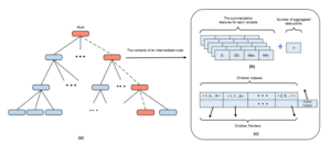
Figure 1: The multi-resolution structure (a) Updating the multi-resolution tree (b) The summarization features (c) The mapping table

The tree is an efficient structure in which summarization features at high levels can be computed from features at low levels without rescanning the original raw data. This is useful for incremental updating. Also, the tree provides quick reference links between its levels to support multiresolution aggregation. Searching the tree structure is faster than searching the massive raw dataset.

All data records are aggregated at each level of the tree. Aggregations are performed on all variables at the same time. This multi-resolution aggregation reduces the number of tree nodes and provides the trade-off between efficiency and accuracy. The user can choose the appropriate level of aggregation. Typically, navigation is a top-down process from the top to lower levels.

Each intermediate node holds a mapping table and a set of summarized statistical measures. The mapping table, Fig.1(c), contains a set of entries that hold node indexes along with their corresponding pointers and is used for linking a node with its parent and children nodes. The mapping tables helps to reduce the I/O operations. For instance, to access a desired child node from its parent, we start by searching the parent’s mapping table to check if the index of the desired child is available.

3.1. Tree Node Index and Mapping between Nodes

A tree node is a hyperrectangular area that is specified by an interval in each dimension. Each interval has a unique index number that distinguishes it from other intervals. Consequently, each node has a set of index numbers corresponding to its intervals in all dimensions. We call this set a node index. The node index is used to identify the exact nodes in the tree to be called and uploaded to the main memory.

A mapping function, f({v₁,v₂,…,v_d}) = {name_l}^h_l=1 is used to generate the node index from incoming data point {v₁,v₂,…,v_d}, where v_i is the value of variable i, and name_l is the node name at level l. Each name is a tuple of the form hl, I₁, I₂,…, I_d i, where l is the tree level and I_i is the region number of variable i. The availability of the node names for incoming data point along with mapping tables, which consist of child nodes indexes, helps to assign the incoming data point to its corresponding nodes without searching the tree. Instead, it uploads only the required nodes for updating. See section III (c) for the detailed procedure.

3.2. Sufficient Statistical Measures

Multiple statistical measures can be collected on data points aggregated in a region. The set of statistical measures should be expressive enough to answer most data queries. Since each data mining algorithm needs different statistical measures, we need to find common statistical measures for all or most of the algorithms to ensure that the proposed structure can be used by these algorithms. Extracting sufficient statistical measures of the aggregated data is crucial to provide information to data analysis algorithms. In addition, efficient analysis of streaming data requires incrementally updating of these statistical features.

For each data node, we collect number of data points, sum of data values, sum of squared data values, as well as minimum and maximum values along each variable (n,S _p,SS _p, Min_p, Max_p) in this node. We collected these measures inspired by BIRCH [31]. These five statistical measures are small in size and can be incrementally updated.

Basic statistics like mean, variance, and standard deviation can be incrementally and directly computed from these statistical features. Other features such as variables correlation and variable distribution can also be computed. We assume that the data is uniformly distributed inside each region of the variable.

These measures provide enough information to compute cluster means, sizes, and distances in different modes. In addition, Euclidean, Manhattan, L1 and L2 distances between cluster centers, and average inter-cluster distances can also be computed. This information is useful for clustering algorithms and similarity-based learning. As we will discuss in Sections IV and V on learning algorithms, other measures such as likelihood, conditional probability, and dynamic splitting can be calculated using the collected statistical measures.

3.3. Implementation and Performance Analysis

The proposed multi-resolution structure is a tree like structure. Its implementation and updating is a top-down process, starting from the root node towards the leaf nodes. Algorithm 1 explains the procedure of implementing and updating the multi-resolution structure. Inputs to the algorithm are the desired number h of levels in the resulted tree structure, expected maximum and minimum values for each variable along with a matrix W of region width for each variable at each level in the tree.

The implementation requires a single scan of the training dataset.

To insert a new data record, the algorithm uses the index keys generated by the mapping function and starts at the root node to find an entry that matches the first index key. If the entry is found, the algorithm updates the corresponding node statistical features. In case the entry is not found, the algorithm creates a new entry in the root mapping table to hold the index key. The algorithm then creates a new node, associate it with the newly created entry, and initialize the node statistical features. The algorithm repeats this process until it reaches the leaf node.

The worst performance of the proposed structure occurs when the tree has the maximum number of nodes. We assume that the number of regions for each variable at a level in the tree doubles in the next beneath level. In this case, each node has a maximum of 2^d child nodes. The total number of nodes in the tree with h levels and one root node is:

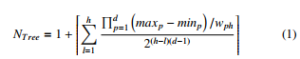
where w_ph ∈ W, is the regions width for variable p at level h. The values max_p and min_p are the maximum and minimum values of variable p respectively.

The proposed multi-resolution tree is an efficient structure since it avoids uploading and searching all tree nodes during insertion and updating. Insertion one data points calls only (h + 1) nodes. Empirically for streaming data, the consecutive data points fall within the same range of values which means that they will be aggregated into the same nodes. Therefore, disk caching helps to reduce disk operations. Implementing the multi-resolution tree does not create empty nodes with no data.

To analysis the worst case to implement the multi-resolution structure, we assume the data of N points is scattered all over the regions and no region left empty. In this case, each node has the maximum number of children and thus the multi-resolution structure has the maximum number of nodes. The implementation of such case costs ONd(R + (h − 1)2^d) where R is the number of entries in the root’s map table, and (h − 1)2^d is the cost to search the map tables of visited nodes. Since h is relatively small value, the cost become ONd(R + 2^d).

Fig. 1 (a) illustrates how Algorithm 1 works. To insert a data record, only the red nodes, one at each level of the tree, are visited and uploaded. The dotted links represent the algorithm traverse and progress from the root to a leaf node.

4. Bayes Data Classification

Class probabilities are essential for Bayesian classifiers, hidden Markov model (HMM), and in defining entropy, gain ratio, and Gini index for decision trees. Naive Bayes is a classification model based on conditional probability. By including class attribute as a regular attribute in building the multi-resolution tree, we can calculate conditional class probabilities from the multi-resolution tree without accessing individual points in the training dataset.

The class attribute, also called the response variable, is a categorical attribute that has a finite number of labels (values). We can divide the class attribute into regions where each region is a unique class label. There is no aggregation applied on the class attribute and it maintains the same set of regions at all levels in the multi-resolution tree. Unlike continuously values variables, no numbers assigned for its regions. Those regions are indexed by their labels.

Given a N×d dataset with the class attribute C = {c₁,c₂,…,c_m}, where m is the number of distinct values of class labels, the number of leaf nodes at level h is:

All data points that are aggregated in a leaf node belong to a single class. Aggregating data points from different classes in one node leads to reduce the number of nodes in the multi-resolution tree and then reduce the storage needed for the tree. However, it consumes more memory and increases the number of I/O disk operations. For example, if parent node aggregates data points that belong to two classes A and B, there is a chance that only one child node has the data points of class A and the rest child nodes have data points belong to class B. Consequently, accessing child node of class A requires to upload all child nodes to memory to find that node of class A.

Computation of class probability from the proposed tree structure requires a single scan of the tree. The highest level in the tree maintains the same information of other levels but it is the most aggregated and compact level. The number of child nodes of the root is much less than the number of data points in the training dataset. Thus, the computation of class probabilities from the highest level in the multi-resolution tree consumes less memory and more efficient than working on the very large training datasets.

Given E = {e₁,e₂,….,e_k}, a set of child nodes of root in the multi-resolution tree that aggregates dataset with the class attribute

C = {c₁,c₂,…,c_m}. The probability of a class c_j, c_j ∈ C and 1 ≤ j ≤ m can be computed by :

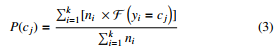
n_i,y_i are the number of aggregated data points and class label of node e_i, F takes value 1 if y_i = c_j and 0 otherwise.

Naive Bayes, Eq. (4), uses class probability for classification. It requires scanning all data points in the training dataset to classify one unknown point, under the assumption that the variables are independent. Suppose continuous variables are normally distributed, it requires to computes the likelihood for a continuous variable using Eq.(5). Then, finds the estimated class label yˆ based on the Bayes theorem that computes class probability P(C) for all classes and assigns the class label c_j with the highest posterior probability to unclassified point x.

The likelihood requires a scan of all points in the training dataset to find the conditional mean, variance and standard deviation to classify a single unknown point. The proposed multi-resolution structure provides an efficient way to compute the conditional mean, variance, and standard deviation of continuous variable p. It requires to scan the nodes of the highest level in the tree only once to compute these conditional features for each class c_j separately, as shown in Table I.

Table 1: Conditional Features Computation for Variable p and class j

Consequently, any classification algorithms based on this computation of class probability can work efficiently without loss in accuracy to cope with the large scale data and streaming data. The multi-resolution Naive Bayes algorithm, which accepts the multiresolution tree as input, has been implemented using Java JDK 13. We have tested the algorithm on eight artificially generated datasets, each set has two continuous variables and binary class label. The multiresolution structured implemented from the training set, 80% of the raw dataset, and the remaining 20% used as a testing set. We have compared the results of applying the multiresolution Naive Bayes on the root level of the multiresolution structure with the results of applying the traditional Naive Bayes algorithm on the raw datasets. Experimental results are given in figure 2. The results show that the multi-resolution Naive Bayes is 25% faster on average than the algorithm that works on raw data sets while keeping the same accuracy of classification.

Figure 2: Comparison of the computation time between multiresolution Naive Bayes (MRNB) and raw data Naive Bayes (NB) algorithms for eight datasets

5. Entropy Discretization Overview and Challenges

We present another application to speed up learning algorithms that sort and search the dataset multiple times to produce an optimal solution. In this section, we propose a high speed and incremental technique for entropy discretization of continuous variables using the multi-resolution structure. The high speed, representative, and incrementally updated structure helps to generate entropy discretization efficiently and effectively for big data and streaming data.

5.1. The Motivation

Several miming and learning logarithms iteratively split the dataset as part of their learning models. Examples of these algorithms are Bayes Belief Network (BBN) classification for continuous data [39], KD-tree used in nearest neighbor (NN) search [40, 41], and conventional decision tree [42] used for classification. The splitting procedure sorts the variable values and then seeks for the best value to split the variable based on a specific criterion. This procedure is repeated for each variable to find the best point and best variable to split the dataset.

The continuous variable has a vast number of values that make sorting and testing of its values during the splitting procedure a complicated task. Entropy discretization converts the continuous variable into a categorical variable by dividing it into a minimal set of non-equal width regions with minimal loss of information. Applying the splitting procedure iteratively on the small number of regions resulted from entropy discretization is more efficient than the iterative scan of the vast number of data points in the dataset. However, entropy discretization is a computationally expensive and memory consuming technique. It needs to search and test all the variable values to divide it into regions. Consequently, entropy discretization is a prohibitive task on big data as well as on streaming data and requires a fast incremental discretization to cope with updating when new data arrives.

5.2. Entropy Discretization Overview and Challenges

Entropy discretization divides the continuous variable based on entropy. Entropy is a measure of information. Higher entropy means less information loss. It is computed by using the frequencyprobability distribution in Eq.(6).

where x is a value in the continuous variable X.

Dividing the continuous variable into several regions affects entropy in a way that the entropy increases when the number of regions increases. To decide the optimal number of regions, there is a comprise between keeping information and keeping performance. Choosing a large number of regions seems reasonable to ensure high entropy and better representation of the distribution in such data. However, there is a danger of an over discretization where too many regions can be dispensable because it slows the performance. Hong [43] proposed a method to find the optimal number of regions with minimal loss of information. The relationship between the entropy and the number of regions is curve. If we draw a straight line from the origin of the graph to the maximum entropy and the maximum number of regions, the curve will be always above the line. Hong showed that when the curve is most apart from the line, we reach the optimal number of regions. This point is called the Knee point.

Ellis [39] uses Hong method to discretize continuous variables and feeds them to the Bayes Belief Network algorithm. His method starts with dividing the continuous variable into regions and sorting them. Each region has a distinct value of the continuous variable. The method then merges two adjacent regions with the smallest difference of frequency (number of aggregated data points). The process of merge continues until reaching the maximum height point on the curve (Knee point). The Knee point is reached when the change in the number of regions becomes greater than the change in the entropy of the regions. This relation is explained in Eq.(7) in the next section. However, when the number of distinct values is very big, this method of entropy discretization is computationally prohibitive. The time complexity of this method for d continuous variables is O(d(m(log₂m + m²), where m is the number of distinct values. The number of distinct values is very big in some applications like sensor data, human activity recognition, and health care data, where m approaches the number of data points N.

5.3. Proposed Algorithm

We propose a fast entropy discretization technique by using the multi-resolution structure. The proposed technique finds the optimal number of non-equal width entropy regions based on the equal width regions in the multi-resolution structure. The multi-resolution structure has properties such as the hierarchical organization of aggregated data which makes the proposed technique more efficient than working on the massive number of data points in the training dataset to generate the regions of entropy discretization.

The multi-resolution structure discretizes each continuous variable into non-overlapping equal-width regions, each resides on a separate node of the same tree level. The proposed algorithm optimizes this discretization of the variable by merging its regions from two different nodes into one region repeatedly until reaching to Knee point.

Algorithm 2 explains the proposed entropy discretization technique for a dataset of d continuous variables. For each variable, the algorithm starts working on the parents of the leaf nodes (it can easily be adapted to work on any other level except root and leaves). For each parent, the algorithm merges the adjust regions in the sibling leaves. The new resulted regions are saved into a local file associate with the parent node. This pass is called the local mode. Then, in the global mode, the algorithm uses regions from all local files and merge the adjacent regions from nodes belong to different parents. The final result of the global mode is a set of optimal entropy regions that are saved into a global file for each variable, as shown in figure 4.

The region is represented by its boundary (cut point) and the number of its aggregated data points (frequency). This information is obtained from the statistical features of the node that hosts the region. The statistical features Max maximum value of the region is used as a cut point while n the number of aggregated data points inside the node is used as frequency. To deal with multiple regions, the algorithm uses a list to save the cut points of that regions combined with a corresponding list of their frequencies.

The merge procedure in algorithm 2, that is used in both local and global modes, is iterative. It sorts the regions based on their cut points and runs the following steps:

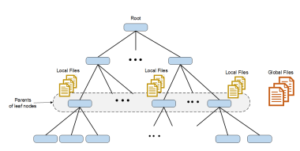
Figure 3: The multi-resolution structure with local and global files, one local file for each variable on every parent node and one global file for each variable

• Compute the entropy, Entr, for current K regions using Eq.(6). In this case, x is a region in variable X. The regions frequencies are used to compute the probability.
• Find two adjacent regions with a minimum frequency difference and merge them. The new cut point of the new region is the greatest cut point of the two merged regions while the new frequency for the new region is the sum of the frequencies of the two merged regions.
• Compute the entropy, newEntr, for resulted K − 1 regions after the merge.
• Compute the rate of change in the number of regions to the change in their entropy using Eq.(7).

The Knee point is proportional to this rate and is reached just before the decrease in this rate. If the rate is decreased, the algorithm stops the merge procedure. Otherwise, the algorithm updates the cut point and frequency lists by replacing the cut points and frequencies of the two merged regions by the cut point and frequency of the new region. The algorithm repeats the last three steps until the rate starts to decrease.

Although the local mode may lead to a little loss in the information due to missing a merge of regions from different parents, the local mode is still important to improve the performance in building and updating entropy discretization. Local mode reduces the sort to only nodes belong to the same parent because these nodes are neighbors to each other and there is a high possibility to merge them. The local mode helps to trigger the global mode only if it is needed, as summarized in Fig 5. After updating the multi-resolution structure due to the arrival of new data points, the local modes are triggered only for the parents of the updated leaves. The local modes for other parent nodes are ignored. If any of the triggered local modes achieves a merge, the global mode will be triggered. Otherwise, the algorithm terminates without global mode because the new data point has not effected the entropy discretization.

Finally, the algorithm outputs a set of global files. The global file contains the optimal number of entropy regions that represent the distribution of a single continuous variable. The set of global files can be used to feed the mining and learning algorithms for efficient and effective learning.

Figure 4: Updating process of multi-resolution structure and entropy discretization

6. Conclusions

In this paper, we have studied fast Bayes classification and entropy discretization of continuous variables using a multi-resolution data aggregation structure for mining and processing of large datasets. The proposed Bayes classification works by getting required conditional probabilities directly from aggregated statistical measures. Entropy discretization works in local and global modes to find the optimal number of non-equal width entropy regions with minimal loss of information based on the equal-width regions of the multi-resolution structure. The multiresolution structure makes the proposed technique more efficient to generate entropy discretization regions than working on the massive number of data points in the big dataset. The resulted entropy discretization regions are saved into files linked to leaf nodes and their parents for fast updates of these regions to cope with streaming data. These files are useful to find the best split point and best split variable for continuous variables that are essential for several learning algorithms that iteratively seek for the optimal variable and value to split the dataset. These algorithms include Bayes Belief Network (BBN) classification for continuous data, KD-tree data structure used in fast nearest neighbor search, and conventional decision trees used for classification.

1. L.-M. Ang, K. P. Seng, “Big Sensor Data Applications in Urban Envi-
   ronments,” Big Data Research, 4, 1–12, 2016, doi:https://doi.org/10.1016/ j.bdr.2015.12.003.
2. B. Fang, P. Zhang, “Big Data in Finance,” in S. Yu, S. Guo, editors, Big Data Concepts, Theories, and Applications, 391–412, Springer International Publishing, Cham, 2016, doi:10.1007/978-3-319-27763-9 11.
3. G.-H. Kim, S. Trimi, J.-H. Chung, “Big-data applications in the government sector,” 2014.
4. L. A. Tawalbeh, R. Mehmood, E. Benkhlifa, H. Song, “Mobile Cloud Comput- ing Model and Big Data Analysis for Healthcare Applications,” IEEE Access, 4, 6171–6180, 2016, doi:10.1109/ACCESS.2016.2613278.
5. H. Zhang, G. Chen, B. C. Ooi, K.-L. Tan, M. Zhang, “In-Memory Big Data Management and Processing: A Survey,” IEEE Transactions on Knowledge and Data Engineering, 27(7), 1920–1948, 2015, doi:10.1109/TKDE.2015.2427795.
6. R. Kune, P. K. Konugurthi, A. Agarwal, R. R. Chillarige, R. Buyya, “The anatomy of big data computing,” Software: Practice and Experience, 46(1), 79–105, 2016, doi:10.1002/spe.2374.
7. M. H. ur Rehman, C. S. Liew, A. Abbas, P. P. Jayaraman, T. Y. Wah, S. U. Khan, “Big Data Reduction Methods: A Survey,” Data Science and Engineering, 1(4), 265–284, 2016, doi:10.1007/s41019-016-0022-0.
8. S. Alwajidi, L. Yang, “Multi-Resolution Hierarchical Structure for Efficient Data Aggregation and Mining of Big Data,” in 2019 International Confer- ence on Automation, Computational and Technology Management (ICACTM), 153–159, 2019, doi:10.1109/ICACTM.2019.8776717.
9. B. H. Brinkmann, M. R. Bower, K. A. Stengel, G. A. Worrell, M. Stead, “Large-scale electrophysiology: Acquisition, compression, encryption, and storage of big data,” Journal of Neuroscience Methods, 180(1), 185–192, 2009, doi:10.1016/j.jneumeth.2009.03.022.
10. H. Zou, Y. Yu, W. Tang, H. M. Chen, “Improving I/O Performance with Adap- tive Data Compression for Big Data Applications,” in 2014 IEEE International Parallel Distributed Processing Symposium Workshops, 1228–1237, 2014, doi:10.1109/IPDPSW.2014.138.
11. A. A. Abdellatif, A. Mohamed, C.-F. Chiasserini, “User-Centric Networks Selection With Adaptive Data Compression for Smart Health,” IEEE Systems Journal, 12(4), 3618–3628, 2018, doi:10.1109/JSYST.2017.2785302.
12. Q. Han, L. Liu, Y. Zhao, Y. Zhao, “Ecological Big Data Adaptive Compression Method Combining 1D Convolutional Neural Network and Switching Idea,” IEEE Access, 8, 20270–20278, 2020, doi:10.1109/ACCESS.2020.2969216.
13. A. Oussous, F.-Z. Benjelloun, A. Ait Lahcen, S. Belfkih, “Big Data technolo- gies: A survey,” Journal of King Saud University – Computer and Information Sciences, 30(4), 431–448, 2018, doi:10.1016/j.jksuci.2017.06.001.
14. D. M. S. Arsa, G. Jati, A. J. Mantau, I. Wasito, “Dimensionality reduction using deep belief network in big data case study: Hyperspectral image classifi- cation,” in 2016 International Workshop on Big Data and Information Security (IWBIS), 71–76, 2016, doi:10.1109/IWBIS.2016.7872892.
15. M. A. Belarbi, S. Mahmoudi, G. Belalem, “PCA as Dimensionality Re- duction for Large-Scale Image Retrieval Systems,” 2017, doi:10.4018/ IJACI.2017100104.
16. J. A. R. Rojas, M. Beth Kery, S. Rosenthal, A. Dey, “Sampling techniques to improve big data exploration,” in 2017 IEEE 7th Symposium on Large Data Analysis and Visualization (LDAV), 26–35, IEEE, Phoenix, AZ, 2017, doi:10.1109/LDAV.2017.8231848.
17. T. Hasanin, T. Khoshgoftaar, “The Effects of Random Undersampling with Simulated Class Imbalance for Big Data,” in 2018 IEEE International Con- ference on Information Reuse and Integration (IRI), 70–79, 2018, doi: 10.1109/IRI.2018.00018.
18. C. K. Maurya, D. Toshniwal, G. Vijendran Venkoparao, “Online sparse class imbalance learning on big data,” Neurocomputing, 216, 250–260, 2016, doi: 10.1016/j.neucom.2016.07.040.
19. W. Song, P. Liu, L. Wang, “Sparse representation-based correlation analysis of non-stationary spatiotemporal big data,” International Journal of Digital Earth, 9(9), 892–913, 2016, doi:10.1080/17538947.2016.1158328.
20. G. Cormode, N. Duffield, “Sampling for big data: a tutorial,” in Proceedings of the 20th ACM SIGKDD international conference on Knowledge discovery and data mining, KDD ’14, 1975, Association for Computing Machinery, New York, New York, USA, 2014, doi:10.1145/2623330.2630811.
21. M. Malhat, M. El Menshawy, H. Mousa, A. El Sisi, “Improving instance selection methods for big data classification,” in 2017 13th International Computer Eng neering Conference (ICENCO), 213–218, 2017, doi:10.1109/ ICENCO.2017 5-2320.
22. J. K. Kim, Z. Wang, “Sampling Techniques for Big Data Analysis,” Interna- tional Statistical Review, 87(S1), S177–S191, 2019, doi:10.1111/insr.12290.
23. S. Garc´ia, S. Ram´irez-Gallego, J. Luengo, J. M. Ben´itez, F. Herrera, “Big data preprocessing: methods and prospects,” Big Data Analytics, 1(1), 2016, doi:10.1186/s41044-016-0014-0.
24. S. Garc´ia, J. Luengo, F. Herrera, “Instance Selection,” in Data Preprocessing in Data Mining, volume 72, 195–243, Springer International Publishing, Cham, 2015, doi:10.1007/978-3-319-10247-4 8.
25. R. M. Kaplan, D. A. Chambers, R. E. Glasgow, “Big Data and Large Sample Size: A Cautionary Note on the Potential for Bias,” Clinical and Translational Science, 7(4), 342–346, 2014, doi:10.1111/cts.12178.
26. Y. Liu, W. Guo, C.-I. Fan, L. Chang, C. Cheng, “A Practical Privacy-Preserving Data Aggregation (3PDA) Scheme for Smart Grid,” IEEE Transactions on In- dustrial Informatics, 15(3), 1767–1774, 2019, doi:10.1109/TII.2018.2809672.
27. M. Tamai, A. Hasegawa, “Data aggregation among mobile devices for upload traffic reduction in crowdsensing systems,” in 2017 20th International Sympo- sium on Wireless Personal Multimedia Communications (WPMC), 554–560, 2017, doi:10.1109/WPMC.2017.8301874, iSSN: 1882-5621.
28. J. Han, “Towards on-line analytical mining in large databases,” ACM Sigmod Record, 27(1), 97–107, 1998.
29. T. Ritbumroong, “Analyzing Customer Behavior Using Online Analytical Mining (OLAM),” 2015, doi:10.4018/978-1-4666-6477-7.ch006.
30. B. W. F. Pan, D. R. Y. Cui, Q. D. W. Perrizo, “Efficient OLAP Operations for Spatial Data Using Peano Trees,” in Proceedings of the 8th ACM SIGMOD workshop on Research issues in data mining and knowledge discovery, 28–34, San Diego, California, 2003.
31. T. Zhang, R. Ramakrishnan, M. Livny, “BIRCH: an efficient data cluster- ing method for very large databases,” in ACM Sigmod Record, volume 25, 103–114, ACM, 1996.
32. M. Ester, H.-P. Kriegel, J. Sander, X. Xu, “A Density-Based Algorithm for Dis- covering Clusters in Large Spatial Databases with Noise,” in Proceedings 2nd International Conference on Knowledge Discovery and Data Mining, 226–231, 1996.
33. K. Mahesh Kumar, A. Rama Mohan Reddy, “A fast DBSCAN clustering al- gorithm by accelerating neighbor searching using Groups method,” Pattern Recognition, 58, 39–48, 2016, doi:10.1016/j.patcog.2016.03.008.
34. Y. Chen, L. Zhou, Y. Tang, J. P. Singh, N. Bouguila, C. Wang, H. Wang, J. Du, “Fast neighbor search by using revised k-d tree,” Information Sciences, 472, 145–162, 2019, doi:10.1016/j.ins.2018.09.012.
35. Y. Hong, Q. Tang, X. Gao, B. Yao, G. Chen, S. Tang, “Efficient R-Tree Based Indexing Scheme for Server-Centric Cloud Storage System,” IEEE Transactions on Knowledge and Data Engineering, 28(6), 1503–1517, 2016, doi:10.1109/TKDE.2016.2526006.
36. L.-Y. Wei, Y.-T. Hsu, W.-C. Peng, W.-C. Lee, “Indexing spatial data in cloud data managements,” Pervasive and Mobile Computing, 15, 48–61, 2014, doi: 10.1016/j.pmcj.2013.07.001.
37. M. Huang, F. Bian, “A Grid and Density Based Fast Spatial Clustering Al- gorithm,” in 2009 International Conference on Artificial Intelligence and Computational Intelligence, 260–263, IEEE, Shanghai, China, 2009, doi: 10.1109/AICI.2009.228.
38. A. Hornung, K. M. Wurm, M. Bennewitz, C. Stachniss, W. Burgard, “Oc- toMap: an efficient probabilistic 3D mapping framework based on octrees,” Autonomous Robots, 34(3), 189–206, 2013, doi:10.1007/s10514-012-9321-0.
39. E. J. Clarke, B. A. Barton, “Entropy and MDL discretization of continuous variables for Bayesian belief networks,” International Journal of Intelligent Systems, 15(1), 61–92, 2000, doi:10.1002/(SICI)1098-111X(200001)15:1(61:: AID-INT4 ) 3.0.CO;2-O.
40. H. Wei, Y. Du, F. Liang, C. Zhou, Z. Liu, J. Yi, K. Xu, D. Wu, “A k-d tree-based algorithm to parallelize Kriging interpolation of big spatial data,” GIScience & Remote Sensing, 52(1), 40–57, 2015, doi:10.1080/15481603.2014.1002379.
41. B. Chatterjee, I. Walulya, P. Tsigas, “Concurrent Linearizable Nearest Neigh- bour Search in LockFree-kD-tree,” in Proceedings of the 19th Interna- tional Conference on Distributed Computing and Networking, ICDCN ’18, 1–10, Association for Computing Machinery, Varanasi, India, 2018, doi: 10.1145/3154273.3154307.
42. A. Bifet, J. Zhang, W. Fan, C. He, J. Zhang, J. Qian, G. Holmes, B. Pfahringer, “Extremely Fast Decision Tree Mining for Evolving Data Streams,” in Pro- ceedings of the 23rd ACM SIGKDD International Conference on Knowledge Discovery and Data Mining, KDD ’17, 1733–1742, Association for Computing Machinery, Halifax, NS, Canada, 2017, doi:10.1145/3097983.3098139.
43. S. J. Hong, “Use of contextual information for feature ranking and discretiza- tion,” IEEE Transactions on Knowledge and Data Engineering, 9(5), 718–730, 1997, doi:10.1109/69.634751.

(Click Here)

(Click Here)