1. Introduction

This paper is an extension of work originally presented in IEEE Nigeria Computer Conference, where a computer software package was developed using Newton-Raphson power flow algorithm [3]. The package was tested with a known solution network and the obtained results are accurate and reliable[3, 8]. Nigerian population is exponentially increasing with the attendant increase in demand for electric power supply proportionally. This becomes a serious task for the power utility companies in the country to meet the huge energy or power demand of the consumers continuously and safely.  Also, power utility companies need to minimize the cost of running the network whether distribution or transmission for smooth, economical and profitable operation of the system. Adding equipment such as generators, lines, buses etc makes the network more prone to faults [3, 4, 8]. Thus, power system network could be interpreted as an interconnection of generators, buses, transformers and lines to give electricity supply to load at several points on the system[3, 4, 8, 11].  However, regardless of the number of load points on the system, the faults should be minimized and the load be made to operate at maximum efficiency with safety so as minimize losses. Therefore, power flow study is employed to study the power system network, and its behavior when it is subjected to any expansion or upgraded for any system.

Power flow studies are tools that are significantly used in system planning and design of power system. It is also used in future expansion and optimization of the existing systems in enhancing reliable performance. The main parameters obtained from typical power flow study include the magnitude and phase angle of the bus bars’ voltages as well as the active and reactive power flowing between the buses [5, 9, 10]. Power flow equations when solved gives the steady state condition of every bus bar voltage of the network. The problem associated with these power flow equations is their non-linearity and difficulty in obtaining solution by mathematical calculation. These non-linear equations are normally solved by iteration techniques [5, 11, 12]. Therefore, power flow solution problems are an iterative process which involves assigning assumed values to the unknown bus bar voltages and subsequent calculation of new voltage values for the bus bars from assumed values for the remaining bus bars with the specified active power and reactive power or voltage magnitude. New set of voltage values for the bus bars are obtained which are eventually used to determine new set of bus bar voltages by a pre-defined algorithm. This iteration process is updated until the voltage changes between the last and just preceding iteration is less than a specified tolerance value for all the bus bars [3, 4, 8, 11]. From literature, most algorithms often result to high number of iterations and hence take long time to complete the required iterations. For a large network, high number of iterations is expected depending on the type of power flow technique and algorithm used. Several iterative techniques are used in power flow studies which include Gauss, Gauss Seidel, Newton Raphson (NR), Fast Decoupled, etc [3, 8]. Many research papers on related topic had been written and published using the above mentioned techniques but their iteration level is high resulting to long period of convergence [3, 8, 9, 12]. Thus, a software package in this regards is predicted to improve the convergence period.

2. Newton – Raphson Algorithm

The technique illustrates a vector ? ∈ ??^? such that,

                     F (?) = 0                                                (1)                                                                                                       where,

                      F = Set of ‘N’ Nonlinear equations.

 In Newton-Raphson (NR) Techniques, the vector of state variable is determined by performing an expansion of equation (1) by Taylor’s series, assuming an initial estimate X (0). Neglecting error in higher order terms of Taylor series; solution for x is obtained using equation (2),

         ? ^(?) = ? ^(?−1) – J^-1 F(? ^(?−1) )                              (2)

where,

                 k = iteration,

                 J = A square matrix of same dimension as ? and F, and its entries are partial derivatives defined as[3,4,6],

where,

         p, q =  Buses.

         ?_?? = Jacobian matrix of equation (1).

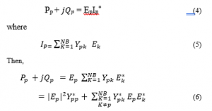
When this mathematical expression is related to power flow solution, then power mismatch is forced to zero via the derivatives of mismatch of the power flow equations. Thus, bus p equation is defined as [1,3],

For p= 1, 2, 3 ………… NB, excluding the slack bus.

In starting iteration, initial voltages often assumed and used. The active power P and reactive power Q evaluated from equation (6) is deducted from the scheduled active power P₂ and reactive power Q_s at the bus. The difference is considered as errors stored. Polar co-ordinates are often used for voltage evaluations. In this approach, the voltage magnitudes and phase angles are treated separately as different variables. Consequently, bus injection equations are differentiated with respect to all variables at each bus. Therefore, the power mismatch for each of the buses are evaluated using equations (7) and (8) [2,7].

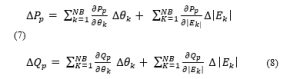
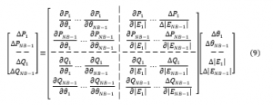
The resulting partial differentials from equations (7) and (8) are put in a Jacobian matrix format so that these equations (7) and (8) are representable in matrix vector form as written in equation (9),

To fasting convergence, multiply voltage corrections by a constant called acceleration factor at each iteration end [3,8,12] as;

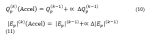
where,  = acceleration Factor,

The common procedures of Newton-Raphson power flow solution are displayed in flowchart shown in Figure 1.

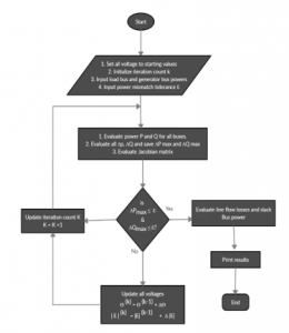
Figure 1:  Common flow process of NR power flow solution

• Developed NRPF Software Package

In solving power flow solution problem using the Newton-Raphson Technique, some computer programs were written to create the software package. The developed NRPF package was implemented for a small power system network using a personal computer (PC) in the paper presented at IEEE Nigeria Computer Conference [3]. The interface of package and it users are interactively designed. The arrangement of the package was done to limit the PC core memory and made possible by overlaying technique.

Overlaying reduced the working memory of the computer and allows the package to be put into modules. With this overlaying, the package operation is in 3 steps and named as;

1. NRPF Supervising module
2. ADESINA 1 Power system data entry and Management
3. ADESINA 2 NR power flow solution.

Only one out of the three modules are allowed to resident in core memory of computer at a time. The Quick Basic language command is used to interface the supervising module (NRPF) to each of the other two modules. Computer programs are coded in Microsoft’s Quick Basic. These two modules are with their respective complete subroutine procedures.

1. Supervising Module (NRPF)

NRPF is more or less act as Controller of the package structure because it allows the user to select which of the two modules is to be executed. At the starting point on computer, the command is C: \>Quick Basic NRPF. This implies loading the module into memory of computer and executes the process. Having activated the module, the computer displays the contents in block 3 of the flow chart in Figure 2

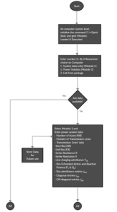
Figure 2a: Flow process of modular operation of the developed software package for NR power flow solution technique.

1. System Data Entry Module (ADESINA 1)

This module permits operational or network data input into computer by the user. It loads and executes the selected option on NRPF’s menu. The Personal computer (PC) interactively ask for the under listed items.

Figure 2b: Flow process of modular operation of the developed software package for NR power flow solution technique continues

1. Number of buses (NB) in the network
2. Number of transmission lines (NL)
3. Transmission line data

    – Start bus, (SB)

    – End Bus, (EB)

– Series resistance, R

    – Series reactance, X

    – Line charging admittance,

4. The bus scheduled active power P_S and reactive powers Q_S. Bus admittance matrix, , are formulated. The non – availability of in – built complex arithmetic functions   in Quick Basic, the real and imaginary parts of  are calculated separately. The admittance matrix, , building algorithms are presented as follows;

The diagonal elements (Y_PP) of the  matrix is calculated by adding lines’ admittances and line charging admittance.

The off-diagonal elements (Y_pq) are the negatives of the admittance buses p and q. Where there are no transmission lines between bus p and bus q, then the off-diagonal element is zero.

The aforementioned data above which already entered as module 1 are stored in data files for future use. This means module 1 do not needs calling since the data are already in memory and kept in data files. Exiting from module 1, the NRPF module is reloaded into memory and executed.

1. Power Flow Solution Module (ADESINA 2)

ADESINA 2 module implements the power flow solution technique. It is loaded into memory and executed provided the data files (ADESINA 1) earlier created had been inputted. When it is noticed that the data files are not in memory then computer gives error signal to show that file data is not yet in computer memory. This imply that, in running this module, the user must ascertain that system data entry module has been executed.

However, it is mentioned earlier that Quick Basic programming language have no in – built complex arithmetic library functions. Due to this lack, power flow solution would need reformulation in rectangular co-ordinates so that parameters in complex form can be effectively manipulated. The module is divided into a main programme and five under listed subroutines.

1. Sub Powers
2. Sub Currents
3. Sub Jacobian
4. Sub Voltage
5. Sub Power flows

The flow process of the program’s logic is illustrated in Figure 2.

3. Description of Nigerian 330kVTransmission Grid

The Nigerian transmission grid is shown in figure 3.  The grid consists of thirty-two buses including   nine generator buses and thirty – four transmission lines. There are three power transformers which are usually the power regulation type. These transformers are usually the power regulation type. Each generation station, depending on its installed generation capacity has a number of generators. Some of the generators in the station are made to supply to the grid, while the remaining ones are considered as reserves. The company’s installed generation capacities are shown in Table 2 [13] . Table 3 [13] shows the number of units of generators found in each station together with corresponding company’s power factor specification. The generating stations have their installed generation capacity and has a number of generator units. Part of installed generators in the station give supply to the grid, while the remaining ones provides the spinning reserves. Available data shows that the total installed generation capacity is 3860MW.

Table 1: Names and Symbols of Buses

Bus No	Bus Name	Bus Symbol
1	Sapele	SPG
2	Osogbo	OS
3	Aiyede	AY
4	Ikeja West	IK
5	Akangba	AK
6	Benin	BN
7	Sapele (L)	SPL
8	Onitsha	ON
9	Enugu	EN
10	Alaoji	ALO
11	Akure	AKR
12	Benin-B	BNB
13	Delta (G)	DTG
14	Ajaokuta	AJ
15	Egbin (G)	EGBG
16	Afam (G)	AFG
17	Portharcourt	PT
18	Aladja	AL
19	Makurdi (G)	MKG
20	Ikom (G)	IKG
21	New-haven	NH

Table 2: Company’s Instilled Generation Capacities [13]

Bus No.	Station Name	Installed Capacity (MW)	Type of Station
1.	Sapele	1020	Thermal
13.	Delta	820	Thermal
15	Egbin (G)	1320	Thermal
16.	Afam (G)	700	Thermal
19.	Makurdi (G)	0	Proposed
20.	Ikom	0	Proposed
Total installed Generation		3860

Table 3: Generator Power Factor Specification for Generation Companies [13]

Substation Location	Number of Units	Power Factor (PF)
Afam I	2	0.80
Afam II	4	0.80
Afam III	4	0.80
Afam IV	6	0.80
Delta I	2	0.80
Delta II	6	0.80
Delta III	6	0.80
Sapele I	4	0.90
Sapele II	4	0.80
Egbin	6	0.80

Table 4: Bus Power and Voltage Specifications in per unit (p.u) [13].

BUS  No	Pg(MW)	Qg(MVAr)	Psp(MW)	Qsp(MVAr)	V(kV)
1	10.2	7.6	0	0	1.0
2	0	0	1.008	0.487	–
3	0	0	1.922	0.897	–
4	0	0	4.55	2.19	–
5	0	0	13.2	5.865	–
6	0	0	2.40	0.75	–
7	0	0	5.10	2.55	–
8	0	0	1.234	0.695	–
9	0	0	2.53	1.226	–
10	0	0	1.638	0.784	–
11	0	0	0.451	0.208	–
12	0	0	1.856	0.896	–
13	8.2	6.15	0	0	1.0
14	0	0	2.20	0.96	–
15	13.2	9.9	0	0	1.0
16	7	5.25	0	0	1
17	0	0	3.39	1.64	–
18	0	0	1.397	0.579	–
19	0	0	0	0	1
20	0	0	0	0	1
21	0	0	0.14	0.57	–

Table 5: Impedance and Shunt admittance of the Transmission Lines in per unit [13]

S/No	SB	EB	Z	YSHT
1	1	7	0          + j 0.0109	0
2	2	3	0.0041 + j 0.0349	0.437
3	2	4	0.0042 + j 0.0344	1.8
4	2	11	0.0037 + j 0.028	0.377
5	3	4	0.0049 + j 0.0416	0.521
6	4	5	0.0003 + j 0.0023	0.13
7	4	6	0.0025 + j 0.0195	4.648
8	4	15	0.0011 + j 0.0086	0.514
9	6	7	0.0005 + j 0.0035	0.832
10	6	8	0.0024 + j 0.0203	1.042
11	6	11	0.0053 + j 0.0483	0.577
12	6	12	0.         + j 0.04	0
13	6	14	0.0035 + j 0.028	1.49
14	7	18	0.0011 + j 0.0095	0.478
15	8	9	0.0148 + j 0.01826	0
16	8	10	0.0023 + j 0.0199	1.048
17	8	21	0.0034 + j 0.0292	0.365
18	9	19	0.0018 + j 0.0139	0.208
19	9	20	0.0015 + j 0.0123	0.616
20	10	16	0.0005 + j 0.0035	0.208
21	12	13	0.0054 + j 0.0173	0.612
22	13	18	0.0011 + j 0.0088	0.135
23	16	17	0.0007 + j 0.0049	0.25

Table 6: Bus Power and Voltage Specifications in per unit

BUS NO	Pg (MW)	Qg (MVAr)	Ps(MW)	Qs(MVAr)	V(KV)
1	10.2	7.6	0	0	1.0
2	0	0	1.008	0.487	–
3	0	0	1.922	0.897	–
4	0	0	4.55	2.19	–
5	0	0	13.2	5.865	–
6	0	0	2.4	0.75	–
7	0	0	5.1	2.55	–
8	0	0	1.243	0.695	–
9	0	0	2.53	1.226	–
10	0	0	1.638	0.784	–
11	0	0	0.451	0.208	–
12	0	0	1.856	0.896	–
13	8.2	6.15	0	0	1.0
14	0	0	2.2	0.96	–
15	13.2	9.9	0	0	1.0
16	7.0	5.25	0	0	1.0
17	0	0	3.39	1.64	–
18	0	0	1.397	0.579	–
19	0	0	0	0	1.0
20	0	0	0	0	1.0
21	0	0	1.140	0.570	–

3.1. Software Application to Sub-Nigerian Transmission Grid.

In this section, the developed software is applied to a Sub-Nigerian Transmission Grid which covers the southern region of the country. This grid network is shown in Figure 3. Per unit impedance and Shunt admittance of the transmission lines in the network diagram of this figure 3 are shown in Table 5.  Other parameters required in data input into computer includes;

The bus scheduled powers for all non-generator buses are already shown in Table 3 above.

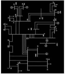
Figure 3: Nigerian 330kV Transmission[3,13]

ADESINA 1 module input data and store in computer memory.  These data include; Number of bus bars, Number of transmission lines, Send-end bus bars number, Receiving-end busbar number, Line impedance, Line Susceptance, Bus scheduled active power  and reactive power . It is followed by the formulation of bus admittance matrix. ADESINA 2 module executes the bus voltage calculations which is initialized by slack bus bar assumed voltage, V = 1.00 + j 0 p.u. The system solution converged in third iteration with mismatched power tolerance, є = 0.001 per unit. The power flow solution of this case study is shown in Table 7 to Table 9.

Table 7: Calculated Bus Voltages of the Network in per unit

Bus	Voltage (per unit)
1	1.0+ j 0
2	1.057 + j 0.062
3	1.051 + j .055
4	1.043 + j .045
5	1.043 + j .045
6	1.027 + j .025
7	1.021 + j .019
8	1.031 + j .029
9	1.047 + j .048
10	1.032 + j .029
11	1.046 + j .049
12	1.024 + j .022
13	1.0     + j 0
14	1.027 + j .026
15	1.0     + j 0
16	1.0     + j 0
17	1.032 + j .029
18	1.022 + j .019
19	1.047 + j .048
20	1.047 + j .048
21	1.031 + j .03

Table 8: Evaluated Bus Voltage Magnitudes, Phase Angles,     Active and Reactive Powers

Voltage (per unit)			Power (per unit)
Bus No	Magnitude	Phase Angle (degree)	Active (MW)	Reactive (MVAr)
1	1	0	0	0
2	1.059	3.357	0	2.203
3	1.052	2.996	0	0.479
4	1.044	2.471	0	3.806
5	1.044	2.471	0	0.065
6	1.027	1.395	0	4.294
7	1.021	1.066	0	0.656
8	1.031	1.611	0	1.228
9	1.048	2.625	0	0.724
10	1.032	1.61	0.001	0.628
11	1.047	2.682	0	0.477
12	1.024	1.231	0	0.306
13	1	0	0	0
14	1.027	1.45	0	0.745
15	1	0	0	0
16	1	0	0.001	0
17	1.032	1.61	0	0.125
18	1.022	1.065	0	0.306
19	1.048	2.625	0	0.416
20	1.048	2.625	0	0.308
21	1.031	1.667	0	0.182

Table 9: Calculated Power Flows between the Buses

Buses		Power Flow (per unit)
From	To	Active	Reactive
1	7	1.746	-1.93
7	1	-1.746	2.004
2	3	-0.221	0.495
3	2	0.221	0.157
2	4	-0.545	0.721
4	2	0.544	-0.063
2	11	-0.516	0.704
11	2	0.514	-0.047
3	4	-0.264	0.744
4	3	0.263	0.37
4	5	0	0.518
5	4	0	0.518
4	6	-1.136	1.278
6	4	1.132	-0.226
4	15	-5.834	5.222
15	4	5.778	-3.786
6	7	-1.936	2.477
7	6	1.933	-0.568
6	8	0.219	0.768
8	6	-0.219	1.14
6	11	0.539	0.592
11	6	-0.541	1.364
6	12	-0.075	1.029
12	6	0.075	0.866
6	14	0.036	0.953
14	6	-0.036	0.946
7	18	0.01	0.09
18	7	-0.01	0.303
8	9	0.112	0.193
9	8	-0.112	0.374
8	10	0.004	0.226
10	8	-0.004	0.329
8	21	0.035	0.28
21	8	-0.035	0.274
9	19	0	0.071
19	9	0	0.071
9	20	0	0.071
20	9	0	0.071
10	16	-9.375	10.947
16	10	9.307	-5.622
12	13	-1.571	0.958
13	12	1.553	-0.902
13	18	2.434	-1.451
18	13	-2.445	3.069
16	17	6.714	-5.047
17	16	-6.768	6.503

4. Discussion of Results

Sapele generating station (Bus 1) of the power system network of figure 3 was chosen as the Slack bus for this analysis. This is because it is one of the sources of supply to the grid. The voltage of generator buses is constrained to 1.0 < 0 per unit.

In Table 8, the magnitude of the bus voltages varies from 1.021 to 1.059 per unit, apart from generator buses that are having 1.00 per unit as constraint value.  The bus bar voltages of 0.95 and 1.05 per unit are recognized as the minimum and maximum voltage values for a standard power system grid [1, 2]. Therefore, buses that are having voltage magnitude whose values falls above 1.05 per unit are regarded as overloaded buses[3,8]. From Table 8, buses 2 (Osogbo) and 3 (Aiyede) falls in to this category of overloaded buses.  Apart from these 2 bus bars, the calculated voltages of other bus bars in the grid are within the allowable range and therefore such bus bars are not overloaded. Overloaded busbars are often experienced due to high electricity demand as well as long distance between the busbars and the supply sources (generating stations). However, it is explicit in the study that two generation sources are not presently existing in the Nigerian power utility 330kV grid, but they are proposed for future expansion. These generation sources are Makurdi (MKG) and Ikom (IKG).

Table 9 shows the network flow pattern of the power flow solution results. It could be seen that these results justified a steady state condition of the grid because the transmission lines are not overloaded. Giving a clear picture, Table 9 illustrates the flow of active and reactive power from bus bar 2 (Osogbo) to bus bar 3 (Aiyede) measured at Aiyede are – 0.221MW and 0.495MVAr per unit respectively. But measuring the returns at Osogbo, the active and reactive powers are 0.221MW and 0.157MVAr per unit respectively which shows that the active power loss on the line is negligible. While lesser reactive power flow is measured at Osogbo, signifying losses.

Also, from Table 9, the Total Power Loss is obtained to be -0.220 + j27.054 per unit while Table 2 shows that the total generation installed capacity is 3860MW. However, it’s rare to have generation companies operating at an installed generation capacity. Therefore, it is assumed in this study that 75% of installed generation capacity is the generation level of the grid network for Nigeria. Consequently, 2895MW being 75% of installed generation capacity and of course the country generation level. From the above, total active power loss is 0.22 per unit which implies 22MW energy loss. Base on this value and generation capacity, the percentage energy loss in this network becomes 0.76%. This mean that energy lost in the network is very little and negligible. The results in table 9 indicates that the slack bus power S₁ is 1.746 + j2.004 per unit at Sapele Generating station while the power  S₂ at bus just immediately after the generation bus  termed Sapele load bus is 1.934 + j0.658 per unit. It is observed that S₂ is greater than S₁ because power S₁ has already been stepped up due to the applied step-up transformer that jacked the generated voltage up for transmission purposes.

In addition, the power utility data shown in table 2 shows that the installed generation capacities (active power) in Megawatts for bus bar 1 (the slack bus) is 1020MW (or10.20 per unit). While, the power flow solution results shows that the slack bus power (active) is 1.746 per unit, which of course is lower than the installed generation capacity of 10.20 per unit. This, however, confirms that the use of bus 1 as the slack bus is realistic. The power flow solution converged at eight iterations and the results obtained are quite reasonable, interpretable and reliable. This makes the software package better compared to previous research works where power flow solution either converged at high iteration level or the system did not converge at all leading to no solution.

It was observed that the following transmission lines are either having high reactive power than the active power or both powers are having almost the same values. The affected lines include; line 1-7, 2-4, 2-11, 4-6, 6-7, 10-16, 13-18 and 16-17. This condition is not tolerated in power system as it causes system instability. Therefore, installation of Capacitor bank or other means of absorbing reactive power on those lines is highly recommended to power utility management.

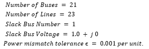
5. Conclusion

This paper presents an application of the developed NR software package to the power flow analysis of Nigerian 330 kV regional power utility grid. The grid consists of 21 buses and 23 transmission lines. Often, a bus bar, preferably a generator bus bar is used as slack bus. Consequently, bus bar 1 (Sapele bus bar) was chosen as the slack bus and its voltage is 1.0 < 0 per unit for this analysis.  The voltage of the voltage controlled bus bars (or generator) were also constrained to 1.0 < 0 per unit.  The results of the analysis converged at the third iteration. This early convergence of the NR solutions satisfied the theoretical reports of Newton – Raphson iterative algorithm. In addition, early convergence may not also be unconnected with the use of real life power system grid having reliable operational parameters or data.  The results of the power flow analysis for this Nigerian 330kV regional transmission grid are presented and discussed. These results are accurate and reliable. The transmission lines with high reactive power will deserves an installation of equipment that could reduce or control the reactive power on the lines.  On the same note, the bus bars with voltage values not fall within the specified range would require the special attention of the power utility company; in this case, Transmission Company of Nigeria (TCN). Furthermore, the package can also be applied to determine the stability of medium voltage distribution feeders.

Conflict of Interest

The authors declare no conflict of interest.

Acknowledgment

The authors sincerely appreciate the Transmission Company of Nigeria (TCN) for providing the data used in this research work.

1. A. Abdulkareem, Power Flow Analysis of Abule-Egba 33-kV Distribution Grid System with real network Simulations., IOSR J. Electr. Electron. Eng. 9 (2014) 67–80.
2. I.A. Adejumobi, G.A. Adepoju, K.A. Hamzat, Iterative Techniques for Load Flow Study: A Comparative Study for Nigerian 330kv Grid System as a Case Study, Int. J. Eng. Adv. Technol. 3 (2013) 153–158.
3. L.M. Adesina, J. Katende, G.A. Ajenikoko, Development and Testing of Q-Basic Computer Software for Newton-Raphson Power Flow Studies, in: 2019 2nd Int. Conf. IEEE Niger. Comput. Chapter, 2019: pp. 1–6.
4. R. Alqadi, M. Khammash, An Efficient Parallel Gauss-Seidel Algorithm for the Solution of Load Flow Problems, Int. Arab J. Inf. Technol. 4 (2007) 148–152.
5. J. Chakavorty, M. Gupta, A New Method of LoadB_ Flow Solution of Radial Distribution Networks, in: 2011.
6. H.-C. Kim, N. Samaan, D.-G. Shin, B.-H. Ko, G.-S. Jang, J.-M. Cha, A New Concept of Power Flow Analysis, J. Electr. Eng. Technol. 2 (2007).
7. M.A. Kusekwa, Load Flow Solution of the Tanzanian Power Network Using Newton-Raphson Method and MATLAB Software, Int. J. Energy Power Eng. 3 (2014) 277.
8. L.M. Adesina, O. Ogunbiyi, G. Ajenikoko, Newton-Raphson Algorithm for Power Flow Solution and Application, 9 (2020) 1–17.
9. V.K. Shukla, A. Bhadoria, Understanding Load Flow Studies by using PSAT, in: 2013.
10. S. Singh, Optimal Power Flow using Genetic Algorithm andParticle Swarm Optimization, IOSR J. Eng. 2 (2012) 46–49.
11. S. Singh, Load Flow Analysis on Statcom Incorporated Interconnected Power System Networks Using Newtonraphson Method, IOSR J. Electr. Electron. Eng. 9 (2014) 61–68.
12. M. Syai’m, A. Soeprijanto, Improved Algorithm of Newton Raphson Power Flow using GCC limit based on Neural Network, Int. J. Electr. Comput. Sci. 12 (2012) 7–12.
13. Transmission Company of Nigeria, Line parameters, Bus specified power and voltages, Annu. Mag. Natl. Grid. (2014).

(Click Here)

(Click Here)