1. Introduction

Demand Side Management (DSM) has been in practice from the 20th century. Initially, DSM was implemented by replacing older equipment with a newer one for improved efficiency. DSM effectively reduces the gap between supply and demand with the help of various services. DSM is performed by suggesting adjustment in the electricity consumption of the customer to produce desired changes in the power distribution system. Some DSM strategies used to alter customers’ load profiles involve load shedding, valley filling, peak clipping, flexible load shape, strategic load growth, strategic conservation and load shifting [1]. The final load profile for each system depends on the operational requirement of the system. Performing DSM has the same objective to minimise customers’ utility bills and to reduce Peak to Average Ratio (PAR) by taking up different pricing models in many researches. By performing DSM, electrical infrastructure can be utilised effectively, and new investments on the same can be deferred. Price billing schemes are an important aspect of performing DSM. In recent times, instantaneous load billing scheme has been used to perform DSM. By implementing this billing scheme, the price at each hour can be changed depending on the aggregated load at that hour.

A quadratic cost function has been used with the motive of reducing the total cost and minimize PAR with a simple billing mechanism for the subsequent period is proposed in [2]. This does not consider peak classification during the day, making it unfair to the customer by billing them similar at all times of the day based only on energy consumption. Some pricing models have been introduced and mapping between retail users and wholesale electric prices is portrayed in [3]. The motive was to improve utilization of cumulative generated energy and reduce energy cost by wholesale mapping of energy requirement [3]. A polynomial cost function with time-dependent coefficients has been used in [4]. The focus was to find the aggregated energy consumption and the selfish customers would modify their energy consumption in order to reduce their energy prices. The time slots have been classified in [4] as on peak, mid-peak and off-peak. Coefficients are time-dependent and are assigned based on the peak classification. The coefficients are based on the currency used in the billing.

A system with industrial, commercial and residential loads have been considered to perform DSM in [5] and hourly costs were paralleled with the costs in [6]. In [5], a logarithmic pricing model was used to compute the energy consumption price and a load shifting based on average cost was devised to perform DSM. The hourly prices were lower when compared to the strategy by [6] which uses a heuristic algorithm to minimise utility costs. [2]-[6] are pivotal to this work as a mathematical pricing model for energy consumption is a significant element for performing DSM.

DSM using strategic conservation is portrayed in [7]. In the study, some customers with the presence of Distributed Generators (DGs) were considered. The key highlights of the study were bi-directional energy flow from customer to grid, incentives and balancing, mass-produced renewable energy. In [8],  discharge of Plug-in Hybrid Electric Vehicle (PHEV) during peak demand was used for DSM. Since different utilities use different pricing methodologies, the concept of cost efficiency as a metric to determine the consumption efficiency is explained in [9]. Home Load Management Systems (HLM) used to achieve residential load management, without focusing on electricity pricing has been discussed in [10]. The concept of coordinated demand response of residential customers in a smart grid has been highlighted. A price model as a ratio of total connected load at that instant to the total aggregated load through all time slots is proposed in [11]. It emphasizes on analysing a realistic situation by considering realistic consumer behaviour to determine the participation of the consumer in DSM. Though the work mentions to account for the realistic situation, deviation of load demand from the forecasted data has been over looked while performing DSM.

A standalone, Hybrid energy source with a combination of wind and solar energy has been designed to electrify a village in India in the study performed in [12]. The design aspects included solar irradiation and wind speed and the objective was to optimize the size of the energy source without affecting the performance of the same. In [13], planning of distributed sources such as distributed generators and shunt capacitors to achieve objectives on technical, economical and societal levels are discussed. Expansion of a micro-grid due to increasing load demand are discussed in [14] with wind turbines, Solar energy source, and batteries. The expansion is carried out in an isolated micro-grid and load forecasting with uncertainties are considered in the research.

In this work, two systems are considered: (i) IEEE 24 bus Reliability Test System (RTS 24) with integrated Windmills [15] and (ii) an institutional energy consumption model with integrated solar panels. Any deviation in the load demand from the forecasted base load is taken into account in the proposed pricing model. This makes the proposed pricing model realistic and practical since load demands are dynamic and seldom match with the forecasts. A polynomial cost function in which coefficients are based on off-peak, mid-peak and on-peak hours from a previously referenced research is also considered and analysed. Load shifting algorithm has been developed to reduce the deviation of hourly load demand from the fixed base load. This has proved to reduce consumers aggregated energy cost for the day and to acquire a flat load profile. This will also reduce PAR and enhance the efficiency of the power system.

2. System Model

Two systems were considered to apply the proposed method. It has been assumed that all the consumers were equipped with HLMs (Home load management systems) or smart meters. IEEE 24-bus reliability test system (RTS 24) with wind energy source of 200MW at six different points in the grid is considered as system 1. Hourly load demand for System 1 is acquired from [15] and the wind scenarios are acquired from [16]. An institution in which a connected load of 4000kW and decentralised solar power plant of an installed capacity of 1.25MW is considered as system 2. Since, an institutional load is considered, all loads are assumed to be shift able during any period of the day.

The RTS – 24 bus system has been considered since it has installed wind energy, which is operational for the entire 24 hours of the day. Since load considered in the RTS 24 bus system is more flexible in contrast to the institutional load considered, it offered a better scope for analysis.

Assuming load demand for future ‘m’ operational periods has been forecasted to perform Demand Side Management. The consumption of energy for ‘m’ time slots can be formulated for any random customer ‘j’ as

where  is the consumption of energy at the m^th hour by customer ‘j’. The energy profile of the consumer is subject to a maximum and minimum constraint.

where   is the maximum energy consumption limit at hour ‘m’ and  is the minimum energy consumption limit at hour ‘m’.

Energy generation from the renewable energy source is also assumed to be forecasted beforehand to perform DSM. The renewable energy output can be formulated as

where  is the energy output from the installed renewable source at the m^th hour by customer ‘j’. It is assumed that the solar plant installed in System 2 can generate energy only during the day time.

3. Problem Formulation

The aim of the study is to minimise energy consumption bills of the consumer without affecting their routine in terms of energy usage.

The suggested DSM considers systems with installed renewable sources. By considering generation from renewable sources, the effective demand from utility reduces. Thus, the cost will also reduce in this case. Energy consumption from the utility can be mathematically computed by

Where  is the energy requirement from the utility for customer ‘j’ at the m^th hour.

A pricing model has been proposed and is compared with a realistic polynomial pricing model [4]. The pricing models have been incorporated in the proposed Demand Side Management. The polynomial cost function [4] used was

where Lh is the hourly load in kWh or MWh, price parameters are given as

4. Proposed Price Model

The suggested pricing model is based on the fixed base load of the system for the particular day and deviation of hourly energy consumption from the base load at each time period. The suggested pricing model can be formulated as

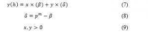
where  is the energy consumption of the consumer at the m^th hour and ‘x’ & ‘y’ are the cost coefficients. ‘y’ is a time dependent factor and is assigned based on peak timings. ‘ ’ is the deviation of hourly energy consumption from the base load ‘ ’. This cost function is more appropriate for DSM, as utility bills of the consumers can be minimised by offsetting the deviation of the energy consumption at that time slot by different methods and services. This price model has been developed from the polynomial cost function and indicates energy consumption prices in cents per kWh or MWh used.

The proposed pricing model possesses important features that are essential for an energy pricing model to be used in DSM. It is a convex cost function; it rapidly increases with an increase in hourly energy consumption.

A generic DSM algorithm has been proposed for any system with forecasted energy generation from the renewable energy source, forecasted load demand at each time slot and a base load of the system.

5. Proposed DSM and Load Shifting Model

Proposed DSM includes energy generation from renewable source installed in the system. By doing so, energy consumption of the consumer from the utility will reduce. This will reflect on the utility bills of the customer for the same energy requirement. The above-discussed cost functions are incorporated to evaluate the utility bills for the customers against their energy usage. A load shifting algorithm has been developed to minimise the hourly deviations at certain time slots. Flowchart for the proposed DSM is shown in Figure 1.

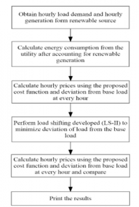
Figure 1: Proposed DSM

A load shifting method is developed to offset the deviation of the load demand from the fixed base load in the time slot under consideration. Load shifting is one among many DSM strategies, where loads from certain time slots of the day are shifted to other time slots to reduce peak demand without creating a new peak at a different time slot. Controllable and non-controllable (critical loads) loads are the two types of loads present in a system. Controllable loads are loads that can be shifted without any constraint and non-controllable loads are those that cannot be shifted [1].

Peaks timings are considered from [4] and each time in a day has been classified as On-peak, Mid-peak, and Off-peak based on the load forecast at that hour. The developed load shifting algorithm aggregates the loads exceeding the base load at each time slot within the peak timings and equally spreads the loads within the peak classifications.

Time slots at on-peak, mid-peak and off-peak is taken as m1, m2, m3 respectively. Fixed base loads at on peak, mid-peak and off-peak are assumed as B1, B2, B3 respectively. The aggregated load at on peak, mid-peak and off-peak periods are given as

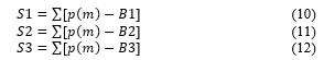
where S1, S2, S3 are the aggregated load that exceeds the base load in each peak period and  is the load demand of the consumer in m^th hour.

Figure 2: Load Shifting Algorithm

Load to be shifted from on-peak, mid-peak and off-peak can be formulated as

where  depict the loads that needs to be shifted within on-peak, mid-peak and off-peak hours respectively. The load demand of the consumer at each peak period after performing the shifting can be formulated as

here,  represent the load demand at on-peak, mid-peak and off-peak hours after performing load shifting.

The developed load shifting algorithm is represented as a flowchart below in Figure 2.

6. Numerical Results

Numerical results of the proposed DSM are presented and are compared with polynomial pricing model [4]. The entire time frame under consideration has been classified into on peak, mid-peak and off-peak hours. ‘a’ in the polynomial cost function and ‘y’ in the proposed cost function is set as 0.003 from 12 Midnight to 7AM (Off-peak), as 0.004 from 7AM to 4PM & 10PM to 12 Midnight (Mid-peak) and 0.005 from 4PM to 10PM (On-peak), ‘b’ and ‘c’ are set as 1 and 0 respectively for all M m.

The proposed DSM has been carried out on System 1 (RTS 24). System data [15], Load management including the renewable generation and load shifting is shown in Figure 3.

Figure 3: Proposed DSM on System 1

For System 2, peak timing has been classified in a slightly different manner taking into account the consumption pattern of the institutional load. Off-peak from 12 Midnight to 6 AM & 10PM to 12 Midnight; mid-peak from 9AM to 5PM and on-peak from 6AM to 9AM & 5PM to 10PM.

The proposed DSM was carried out on System 2. System data and Load management after including energy generation from the renewable source and load shifting are shown in Figure 4.

Figure 4: Proposed DSM on System 2

Hourly energy prices for System 1 and System 2 are calculated using the proposed pricing model and compared with the polynomial cost function [4]. Energy prices at each time slot for System 1 before and after load shifting, by polynomial and proposed cost functions are shown in Table 1.

Table 1: Hourly energy prices by polynomial and proposed cost function on System 1

Time slots	Hourly load in MWh	Polynomial cost function [4]		Proposed cost function
		Before load shifting	After load shifting	Before load shifting	After load shifting
1 2 3 4 5 6 7 8 9 10 11 12 13 14 15 16 17 18 19 20 21 22 23 24 Total:	978.6 901.2 857.2 860.2 891.6 920.4 1250.8 1524.4 1688.1 1625 1572.8 1519.6 1502.3 1508.3 1452.2 1424.1 1470.3 1453 1486.7 1437.5 1362.1 1227.9 1045 874.8 30834.1	2.9358 2.7036 2.5717 2.5807 2.6748 2.7612 3.7524 6.0976 6.7525 6.4999 6.2911 6.0783 6.0092 6.0332 5.8087 5.6963 7.3516 7.2648 7.4337 7.1877 6.8107 6.1396 4.18 3.499 125.1141	2.8543 2.8543 2.8543 2.8543 2.8543 2.8543 2.8543 5.7223 5.7223 5.7223 5.7223 5.7223 5.7223 5.7223 5.7223 5.7223 7.0313 7.0313 7.0313 7.0313 7.0313 7.0313 5.7223 5.7223 125.1132	6.0634 5.8312 5.6993 5.7083 5.8024 5.8888 6.88 7.6614 8.3163 8.0637 7.8549 7.6421 7.573 7.597 7.3725 7.2601 7.3516 7.2648 7.4337 7.1877 6.8107 6.1396 5.7438 5.0628 164.2091	4.7572 4.7572 4.7572 4.7572 4.7572 4.7572 4.7572 6.6738 6.6738 6.6738 6.6738 6.6738 6.6738 6.6738 6.6738 6.6738 7.0313 7.0313 7.0313 7.0313 7.0313 7.0313 6.6738 6.6738 148.9

It can be observed from Table 1 that with the given cost function using the proposed DSM, hourly costs during on-peak periods are scaled to a price highest of the three followed by mid-peak and off-peak periods. This is detected because of the development of coefficients in the proposed cost function pertaining to peak timings. These coefficients influence the cost of electric power during a given time of the day.

Energy prices at each time slot for System 2 before and after applying the load shifting algorithm are given in Table 2.

Table 2: Hourly energy prices by polynomial and proposed cost function on System 2

Time slots	Hourly load in kWh	Polynomial cost function [4]		Proposed cost function
		Before load shifting	After load shifting	Before load shifting	After load shifting
1 2 3 4 5 6 7 8 9 10 11 12 13 14 15 16 17 18 19 20 21 22 23 24 Total:	686.4 686.4 686.4 686.4 686.4 686.4 672.2 555.1 331.6 35.3 24.4 136.6 -292.9 -144.8 -109.6 90 856.8 484.2 1008 688 944 686.4 686.4 686.4 11456.5	2.0592 2.0592 2.0592 2.0592 2.0592 2.0592 4.0335 3.3304 1.9898 0.1412 0.0976 0.5465 -1.1714 -0.5793 -0.4382 0.3601 3.427 2.9054 6.048 4.128 5.664 4.1184 2.0592 2.0592 51.0746	2.0592 2.0592 2.0592 2.0592 2.0592 2.0592 4.0272 4.0272 4.0272 0.2979 0.2979 0.2979 0.2979 0.2979 0.2979 0.2979 0.2979 4.0272 4.0272 4.0272 4.0272 4.0272 2.0592 2.0592 51.0744	2.5392 2.5392 2.5392 2.5392 2.5392 2.5392 3.7935 3.0904 1.7498 0.3812 0.3376 0.7865 -0.9314 -0.3393 -0.1982 0.6001 3.667 2.6654 5.808 3.888 5.424 3.8784 2.5392 2.5392 54.9146	2.2082 2.2082 2.2082 2.2082 2.2082 2.2082 3.9527 3.9527 3.9527 0.3724 0.3724 0.3724 0.3724 0.3724 0.3724 0.3724 0.3724 3.9527 3.9527 3.9527 3.9527 3.9527 2.2082 2.2082 52.2664

It can be observed from Table 2 that renewable energy generation from the solar installations is higher than the load demand of 13^th, 14^th and 15^th hour. By performing the proposed load shifting ensures effective usage of the generated renewable energy during all time slots in the day. The shiftable loads during other time slots avail the excess energy beyond the demand in these time slots.

It can be observed from Table 1 and Table 2, by the proposed pricing model, aggregated hourly cost after shifting is lesser than the aggregated hourly cost before shifting. The overall cost has been reduced by reducing the hourly deviation by load shifting at certain time slots.

Cost-benefit of the proposed cost function is depicted in Table 3. It is observed that there is a significant cost benefit with the proposed cost function after shifting during the mid-peak and off-peak hours in both the systems where as there is a meagre change in the aggregated cost on the on-peak hours.

It can be observed from Figure 3 and 4, by the proposed DSM, the energy requirement is not compromised, while it is being met efficiently. By performing the proposed DSM, a flat load profile can be obtained for certain timeslot thus improving Peak to Average Ratio.

It is a superior substitute to previously existing instantaneous energy billing models. The customers will not have to downsize their consumption but have to shift non-essential consumption to reap benefit in the proposed DSM. Participation of customers in DSM would increase, to minimize their deviation from the already predicted fixed base load with the knowledge of the deviation from base load from the HLM.

Table 3: Cost-benefit with the proposed Cost function on system 1 and 2

Cost-Benefit of proposed cost function on System 1
Peak Classification	Before Load Shifting	After Load Shifting
On Peak	42.1881	42.1878
Mid Peak	80.1476	73.4118
Off Peak	41.8734	33.3004
Cost-Benefit of proposed cost function on System 2
On Peak	30.2975	31.6216
Mid Peak	4.3035	2.9792
Off Peak	20.3136	17.6656

7. Conclusion

For a successful DSM, pricing model and billing mechanism are crucial. The proposed pricing model based on the deviation of hourly load demand from the fixed base load has been observed to be a better alternative over the other realistic polynomial cost function.

Renewable generation is unforeseeable and, in most cases, influenced by external factors. The generation from the renewable sources can be higher than the system requirements during some periods in a day and by performing load shifting, generation from renewables can be effectively utilised. By adopting the proposed algorithm, the energy requirement of the system from the utility decreases.

The total cost is reduced after load shifting is performed by the proposed cost function. This is due to the fact that by load shifting, the deviation of the hourly load demand from the fixed base load is reduced at certain time slots and increases in some to have a balanced shifting, but generated energy is effectively utilised. Therefore, the aim to reduce consumers’ utility bills are met and peak to average ratio improves by incorporating the proposed DSM.

Conflict of Interest

The authors declare no conflict of interest.

Acknowledgment

The authors would like to thank SASTRA Deemed University for sharing their consumption data and energy generation from their installed solar power plant.

1. B.R. Gupta, ‘Generation Of Electric Energy’ (S. Chand Limited, 2009)
2. A.H. Mohsenian-Rad et al., “Autonomous Demand Side Management Based on Game-Theoretic Energy Consumption Scheduling for the Future Smart Grid,” IEEE Trans. Smart Grid, 1(3), 320–331, 2010, doi: 10.1109/TSG.2010.2089069
3. P. Samadi et al., “ Advanced Demand Side Management for the Future Smart Grid Using Mechanism Design,” IEEE Trans. Smart Grid, 3(3), pp. 1170–1180, 2012, doi: 10.1109/TSG.2012.2203341
4. H.H. Chen, “Autonomous Demand Side Management with Instantaneous Load Billing: An Aggregative Game Approach,” IEEE Trans. Smart Grid, 5(4), pp. 1744–1754, 2014, doi: 10.1109/TSG.2014.2311122
5. B. Saravanan, “DSM in an area consisting of residential, commercial and industrial load in smart grid,” Front. Energy, 9(2), 211–216, 2015, doi: https://doi.org/10.1007/s11708-015-0351-0
6. T. Logenthiran et al., “Demand side management in smart grid using heuristic optimization,” IEEE Trans. Smart Grid, 3(3), 1244–1252, 2012, doi: 10.1109/TSG.2012.2195686
7. I. Atzeni et al., “Demand-Side Management via Distributed Energy Generation and Storage Optimization,” IEEE Trans. Smart Grid, 4(2), 1–11, 2012, doi: 10.1109/TSG.2012.2206060
8. B. Gao et al., “Game-theoretic energy management for residential users with dischargeable plug-in electric vehicles,” Energies, 7(11), 7499–7518, 2014, doi: https://doi.org/10.3390/en7117499
9. J. Ma et al., “Residential Load Scheduling in Smart Grid: A Cost Efficiency Perspective,” IEEE Trans. Smart Grid, 7(2), 771–784, 2015, doi: 10.1109/TSG.2015.2419818
10. A. Safdarian, “Optimal Residential Load Management in Smart Grids: A Decentralized Framework,” IEEE Trans. Smart Grid, 7, (4), 1836–1845, 2016, doi: 10.1109/TSG.2015.2459753
11. Y. Wang et al., “Load Shifting in the Smart Grid: To Participate or Not?,” IEEE Trans. Smart Grid, 7(6), 2604–2614, 2016, doi: 10.1109/TSG.2015.2483522
12. S. Rangnekar et al., “Sizing and performance analysis of standalone wind-photovoltaic based hybrid energy system using ant colony optimisation,” IET Renew. Power Gener., 10(7), 964–972, 2016, doi: 10.1049/iet-rpg.2015.0394
13. N. Kanwar et al., “Optimal distributed resource planning for microgrids under uncertain environment,” IET Renew. Power Gener., 12(2), 244–251, 2018, doi: 10.1049/iet-rpg.2017.0085
14. Z. Wang et al., “Optimal expansion planning of isolated microgrid with renewable energy resources and controllable loads,” IET Renew. Power Gener., 11(7), 931–940, 2017, doi: 10.1049/iet-rpg.2016.0661
15. C. Ordoudis et al., “An Updated Version of the IEEE RTS 24-Bus System for Electricity Market and Power System Operation Studies,” Technical University of Denmark. 2016.
16. Data for Stochastic Multiperiod Optimal Power Flow Problem’, https://sites.google.com/site/datasmopf/, accessed April 2018.

(Click Here)

(Click Here)