1. Introduction

At present times, healthcare sector becomes more common where massive amount of medical data plays a major role. In this view, for instance, precision healthcare aims to assure the proper medication is offered to the appropriate patients promptly by considered different dimensions of patient’s information, comprising variability in molecular trait, atmosphere, electronic health record (EHR) and standard of living [1]. The higher accessibility of medical details brought numerous chances and issues related to healthcare researches. Particularly, discover the interconnections between diverse set of data exist in dataset still remains a basic issue to design effective medicinal models using data driven techniques and machine learning (ML). Earlier studies have focused on linking many data sources for building joint knowledge bases which can be utilized for predictive analysis and discovery. Though former techniques exhibit noteworthy performance, prediction models using ML models are not mainly employed in healthcare sector [2]. Actually, it is not possible to completely utilize the available healthcare data due to its sparsity, high dimensional heterogeneity, temporal dependence, and irregularities. These problems become even more difficult by distinct medicinal ontologies employed for data generalization which frequently include disagreements and inconsistencies. In some cases, the identical clinical phenotype can be defined in several ways along the data [3].

For instance, in EHR, a patient affected by ‘type 2 diabetes mellitus’ could be detected by the use of laboratory test reports of haemoglobin A1C >7.0, occurrence of 250.00 ICD-9 code, ‘type 2 diabetes mellitus’ declared in the free text medical notes, etc. As a result, it is not trivial to harmonize every medical concept to develop a higher-level semantic structure and comprehend their relationships [4]. A widespread method in healthcare researches is to have medical experts for specifying the phenotypes to utilize in an adhoc way. At the same time, the supervised description of the feature space performs poor scaling and ignores the chances of discovering effective patterns.

On the other hand, representation learning approaches permit automatic discovery of representations required to predict it from the actual data. Deep learning (DL) techniques are representation-learning approaches with many stages of representation, attained by integrating simpler but nonlinear models [5]. DL models exhibited better results and attained significant attention in natural language processing, computer vision, and speech recognition. DL models have been introduced in healthcare sector due to its better performance in various fields and fast developments of technical enhancements [6]. Several works have also been carried out on DL model for biomedical sector. For instance, Google DeepMind has initiated schemes to utilize its knowledge in medicinal field. In contrast, DL models have not been broadly validated for a wide range of medicinal issue which can get advantages from its abilities [7] . DL have several ways which can be supportive in healthcare, namely multi-modality data, capability of handling complex, superior performance, and end-to-end learning scheme includes characteristic learning etc. Stepping up these works, the entire DL research study should address many issues describing the features of healthcare info requires to upgrade the patterns and tools which allows DL to combine through healthcare workflows and medical decision support [8] . At the same time, the performance of the DL is mainly based on the hyper parameters such as, learning rate, batch size, momentum, and weight decay, which need expertise and wide-ranging trial and error. As a result, the procedure to determine the optimum configuration of the hyper parameters of a DL is still remains a major issue.

In this view, this paper presents a new hyperparameters tuned DL models for intelligent medical diagnosis and classification. The proposed model is mainly based on four major processes namely pre-processing, simulated annealing (SA) based feature  extraction, recurrent neural network (RNN), gated recurrent units (GRU) and long short term memory (LSTM) based classification and differential evolution (DE) based parameter tuning. A detailed simulation analysis takes place using three benchmark medical dataset namely Diabetes, EEG Eye State and Sleep stage dataset.

2. Related Works

Numerous research methods apply DL to forecast diseases from the status of the patient [9]. Use a 4-layer CNN to identify block of heart failure and chronic obstructive pulmonary disease and demonstrate topmost beneficiary measures. RNN with word embedding, pooling and Long Short-Term Memory (LSTM) concealed unit were applied in Deep Care, an end-to-end deep dynamic network that conclude existing infection declare and calculates upcoming healthcare results. The authors planned to sense LSTM part with a degrade events in handling uneven timed actions (i.e. usually longitudinal EHR). Besides, they included medicinal involvement in the techniques to finding the shapes in a dynamic manner. DeepCare estimates the threat on diabetes in future and psychological healthcare of patient cohort, intervention recommendation, and modelling the evolution of disease [10].

RNN with Gated Recurrent Unit (GRU) are utilized by to design Doctor AI, an end-to-end model which make use of patient’s record to calculate diagnose and medication for successive encounter. The valuation indicated notably higher recall compared to low baseline and good believes by adjusting the resulting method from one body to another without losing large accuracy rate [11]. In other aspects, [12] designed a model to study deep patient representation from the EHR via a 3-layer Stacked Denoising Autoencoder (SDA). They apply this novel version on disease to predict the risk by means of random forest as classification model. The validation have been implied on 76,214 patients comprise seventy eight diseases from various medical domains and temporal window (within 1 year). As a finally result, drastically the deep representation direct to better prediction than utilizing raw EHR or conventional representation learning algorithms (e.g. Principal Component Analysis (PCA), k-means). Likewise, they illustrated that result considerably gets better after accumulating a logistic weakening layer on top of the last AE to modify the whole supervised network.

Likewise, [13] use RBM to discover representation of EHR which exposed a novel concept and established an improved approach for predicting accuracy ratio on diseases count . DL was tested to model nonstop time signals, like laboratory result, towards the usual recognition of definite phenotype. For instance,[14] utilized RNN by LSTM to identify the pattern in multivariate time series of experimental dimensions. Especially, a technique has been trained to classify 128 diagnoses from 13 but unevenly sample experimental dimensions from patients in pediatric Intensive Care Unit (ICU). The result shows a major improvement comparing with some sturdy baselines includes multilayer perceptron skill on the hand-engineered type. Use SDA regularize with earlier facts based on ICD-9 for discovering a featured pattern of physiology in medical time sequence [15].

Use a 2-layer stack AE (without regularization) to design a longitudinal series of serum uric acid measurement to differentiate the uric-acid signature of gout and sharp leukemia [16]. Evaluate CNN and RNN with LSTM unit to foresee the beginning stage of disease only from lab-test measures, presenting enhanced output than logistic regression with handcrafted, medically related characteristics [17]. Neural language deep model are applied to EHR, specifically to study embedded representations of the medicinal proposal, equally as diseases, medication and laboratory test that can be used for testing and estimate. As a pattern, use RBM to find out abstraction in ICD-10 cryptogram on a cohort of 7578 logical health patients for forecasting risks of suicide [18]. A wide plan related to RNN obtains capable effects in eliminating protected health details from medical observations to influence the usual de-identification of free-text patient summary. The calculation for not planned patient readmissions after the discharge in recent times receives concentration as well. In this field, presented Deepr, an end-to-end architecture which supports on CNN, which detect and merge medical pattern in the longitudinal patient EHR for stratifying medicinal threats [19]. Deepr carried out fine in forecasting the readmission in six months and have ability to notice significant and interpretable clinical patterns.

3. Objectives

Differential Evolution (DE) is an optimization algorithm. This study aims to apply DE to tune hyper parameter settings of the deep learning models. The convergence of DE algorithm is evaluated to select optimal hyperparameters on the basis of certain searching process such as crossover, mutation and selection. The enhancement of the accuracy and performance of the proposed model is also determined in comparison with Random search algorithm.

4. The Proposed Model

The working process of the presented model is shown in Figure 1. As shown in Figure, the input data undergoes pre-processing, feature extraction, classification and parameter optimization. Initially, the input data is pre-processed to remove the unwanted data and transform it to a compatible format. Then, SA-FS process takes place to select the useful subset of features. Then, DL models are applied to carry out the classification process. Finally, DE is applied for the parameter optimization of the DL models.

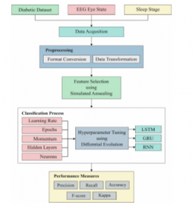
Figure 1: Block diagram of proposed method

4.1. Pre-processing

The major task of data pre-processing is converting the original input data into most intelligible format. As the practical input data is incomplete, there is maximum probability of having error filled data. Thus, data pre-processing is mainly used for transforming the actual data into understandable format which can be applied for next computation. In this approach, pre-processing is carried out in 2 phases such as, Format conversion as well as Data transformation. Initially, format conversion task is conducted when any kind of data type is transformed into .arff format. Then, data transformation is processed with diverse sub-processes as given in the following.

Normalization: This process is applied for scaling the data measures within the specific grade as (-1.0 to 1.0 or 0.0 to 1.0)

Attribute Selection:  Novel attributes are obtained from the given set of variables which is applied for mining task in future.

Discretization: Actual measures of mathematical attributes would be interchanged by conceptual levels.

4.2. SA based Feature Selection Process

SA is defined as a processing model of annealing operation. For physical content, the premise should be filled with massive amount of energy and periodically during the cooling operation. When a solution is applied with minimum criterion value, then it is managed using a degree of minimization as well as a current temperature  for all  iterations [20]. Followed by, the temperature is slowly reduced while limiting the likelihood of accepting inferior solutions. Some of main components of SA for FS are listed as follows.

• The method to generate initial subset;
• The selection of a temperature rank which is defined by maximum , minimum , temperature, and cooling scheme.

5. Methodologies

In this section, three DL models namely RNN, GRU and LSTM   which are applied for classification process has been discussed in the following subsections.

5.1. RNN based Classification Model

RNN belongs to the NN where the output from existing step is induced as input to the next step. In classical NN, every input and output are autonomous; however, the prediction of a data is processed using previous data and no requirement of memorizing the previous data. Hence, RNN is used to resolve these issues with the help of a hidden layer. The most remarkable feature of RNN is hidden state that saves few data regarding the sequence. RNN is composed of a “memory” that records every detail that has to be determined. It applies similar parameters for every input as it processes the similar operation on hidden layers and produces the better outcome. Finally, the difficulty of parameters is reduced on contrary to alternate NN. Here, NN performs the following operations such as RNN transforms the autonomous activations to dependent activations by generating the similar weights and biases for all layers, and minimize the complications of parameters and remember every existing output by providing the result as input to the subsequent hidden layer. Thus, 3 layers are combined where weights and bias of each hidden layer is identical, that forms an individual recurrent layer.

 Training through RNN

The training process involved in RNN is listed as follows.

• A single time step of input is given to the network.
• Determine the present state with the help of recent input and existing states.
• The present h_t forms h_t-1 for future time step.
• The same is repeated on the basis of problem and combine the data from previous states.
• After completing the last current state then it computes the attained result.
• Then result is related to original output where the desired result and an error are produced.
• The error undergoes back-propagation to the network and improves the weights so that RNN it trained.

5.2. LSTM based Classification Process

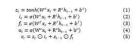
LSTM performs the learning operation over a range of prolonged time intervals. It solves the diminishing gradients problem by replacing periodical neuron using complex structural method named as LSTM unit. The LSTM consists of four neural network layer and three gates (input gate, forget gate and output gate) that are used to control the flow of information. These gates are employed using logistic function in order to calculate the values between 0 and 1. The key elements of LSTM are provided in the following and illustrated in Figure 2.

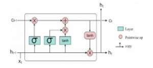
Figure 2: LSTM Model

Input Gate (

        An input gate controls a new value flow into the memory. Forget gate (

 A forget gate removes the information from the cell state which is no longer required to process.  It performs scaling on the internal state of the cell in prior to adding it as input to the cell through the self-recurrent connection of the cell, so adaptively forgetting or resetting the cell’s memory

Output Gate (  

   It is also a multiplicative unit determines the next hidden state from the current cell state.

Cell State (  

  Cell state contains memory unit which maintains all relevant information required for processing. After the gates are closed, data is trapped inside a memory cell. It activates the error signals flowing over several time steps with no consideration of vanishing gradients. The equation of the LSTM units are given below.

5.3. GRU based classification model

The Vanishing-Exploding gradients issue can be solved           using RNN. The major scheme is LSTM. A model with minimum popularity but highly productive variations is named as GRU. In contrast to LSTM, it has 3 gates which do not retain the Internal Cell State. The data saved in Internal Cell State in an LSTM recurrent unit is embedded into hidden state of GRU. The collected data is provided to the subsequent GRU. Some of the various gates of a GRU is defined in the following:

Update Gate (z)

It computes the previous knowledge that has to be conveyed to future processing. It is analogous to Output Gate in LSTM recurrent unit.

 Reset Gate (r)

      It evaluates the older knowledge which has to be discarded. It is analogous to the integration of the Input Gate and Forget Gate in an LSTM recurrent unit.

Current Memory Gate ( )

It is highly applied for GRU process. It is combined into Reset Gate with Input Modulation Gate is a sub portion of Input Gate and applied to establish non-linearity into input and make the input Zero-mean. An alternate reason to make a sub-part of Reset gate is to limit the effect of existing data on recent information which is applied for next computation.

The fundamental task of GRU is related with RNN as defined with few variations between 2 models. Figure 3 shows the structure of GRU model. The inner working process of GRU has gates that change the recent input and existing hidden state. The working of GRU has been discussed as follows. Initially, the input as current input and older hidden state are assumed as vectors. Then, the measures of 3 various gates are computed as follows.

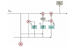
Figure 3: Structure of GRU model

Initially for all gates, determine the parameterized recent input and previous hidden state vectors by processing element-wise multiplication among the assumed vector and the respective weights. Then, Use the concerned activation function for a gate element-wise on parameterized vectors. The list of gates is provided with the activation function. The task of calculating the recent Memory Gate is different from alternate process. Initially, the Hadamard product of Reset Gate as well as previous hidden state vector has been examined. Then vector undergoes parameterization and included to parameterize recent input vector.

The present hidden state is calculated by same vector and dimensions of input are defined. These vectors are indicated by 1. Then compute the Hadamard product of update gate and existing hidden state vector. Also, produces a novel vector by reducing the update gate from ones and determine the Hadamard product of vector present in recent memory gate. Consequently, include 2 vectors for reaching recent hidden state vector.

6. DE based Parameter Optimization Model

The main aim of DL classification model is to optimize the     hyper-parameters namely epochs, learning rate, momentum, hidden layers, and neurons with the application of DE method and results in optimal medical data classification. Here, the parameters exist in these methods are Batch size and count of hidden neurons. The DE model is initialized from first solutions that is produced randomly and tries to enhance the accuracy of emotion classification. The Fitness Function (FF) of DL approach is applicable to perform the estimation and provide the accuracy of medical data classification [21]. DE approach was initially coined by Storn. Generally, DE is mainly applied for parameter optimization as well as real value functions. It is a population oriented searching that has been employed extensively for frequent searching process. Currently, the efficiency of DE is represented in various applications like strategy adaptation for global numerical optimization and FS for healthcare diagnosis. Similar to Genetic Algorithm (GA), DE models employs the crossover and mutation; however, the equation is improved in explicit manner. The optimization in DE is composed of 4 phases: initialization, mutation, crossover and selection.

Firstly, the primary population has been produced randomly, in which Np implies the population size and  means the recent iteration, where initialization is 0. It is defined for all types of problem space with specific integer ranges constrained by upper as well as lower bounds: , for  1 , 2, , where  denotes the dimension of problem space. The main objective of this model is to optimize the hyperparameters of RNN, GRU and LSTM networks, hence, the dimension of the problem is 2 . Every vector is combined and develops into candidate solution , named as target vector, to the multi-dimensional optimization issue. Secondly, in mutation, there are 3 unique vectors from population  are decided arbitrarily to produce novel donor vector  with the help of mutation function

Where  depicts the constant lies between , 2  defines the mutation factor. It is apparent that, the value of  for all dimensions are measured adjacent to integer value. Then, in crossover, the trial vector has been determined for all  dimension of target vector  and every  dimension of donor vector  using binomial crossover. Here, the dimension of trial vector is managed by  , cross over rate, that is a user based constant from , 1].

where  refers the even distributed random integer within  , and  represents the shared random value from , 1 . Finally, in selection, the target vector  is related with trial vector , and maximum accuracy is elected and applied for future generation. It is clear that, the selection operation is attained using different deep learning technique, and a vector with effective fitness value is admitted for next iteration. Hence, the last 3 phases are repeated until meeting the termination condition. The entire process of DE based parameter tuning of DL models is provided in Algorithm 1.

Algorithm 1: Differential Evolution with Deep Learning Models (LSTM, GRU, RNN)
Initialization; Population Size (PS), Crossover Rate (CR), Scale Factor (SF), Termination Criteria (TC)
Begin Procedure
while (TC Not Met) do
	For Each individual, target vector, in the PS;
	Mutation: Choose three individuals from the PS arbitrarily    and generate a donor vector using Eq. 9 Crossover: Calculate the trial vector for the ith target vector using Eq. 10 Selection: Apply LSTM, GRU, RNN Algorithm as fitness function f and evaluate If  then Else
	End For
End While
End Procedure

7. Performance Validation

7.1. Dataset used

The performance of the proposed model undergo validation against three benchmark medical dataset namely diabetes, EEG EyeState (UCI Machine Learning Repository) and Sleep Stage dataset (physionet.org). The details of the dataset are shown in Table 1. The first diabetes dataset includes a total of 101766 instances with the existence of 49 features. Besides, the number of classes in diabetes dataset is two, where 78363 instances comes under positive class and remaining number of 23403 instances falls into negative class.

Table 1: Dataset Description

Dataset Type	Description	Values
Diabetes	Number of Instances	101766
	Number of Attributes	49
	Number of Class	2
	Number of Positive Samples	78363
	Number of Negative Samples	23403
	Data source	[UCI Repository]
EEG Eye State	Number of Instances	14980
	Number of Attributes	15
	Number of Class	2
	Number of Class 1	82527
	Number of Class 2	6723
	Data source	[UCI Repository]
Sleep Stage	Number of Subjects	25
	Sex Distribution Male	21
	Sex Distribution Female	4
	Average Age	50
	Average Weight	95
	Average Height	173
	Number of Class	5
	Name of the Class	Wake/S1/S2/SWS/REM
	Data source	[Physionet.org]

Next, the second EEG Eye Sate dataset comprises a total of 14980 instances with 15 features. Among the total number of instances, a set of 82527 instances comes under class 1 and the remaining 6723 instances falls into class 2. The duration time of every recording was 117 seconds. Next, diverse eye states monitored for each recording were added manually. Consequently, the corpus dataset was developed with 14980 instances. Every instance has 14 EEG features and an eye-state class (either 0 for open, or 1 for closed). Additionally, the count of instances with open-eye class in the corpus dataset is 8257 (55.12%), at the time of number of closed-eye type instances is 6723 (44.88%). Moreover, the dataset is applied in massive studies. Hence, 3 of the instances’ (2 open states, and one closed state) values were outliers and it is applicable to remove from classification process. Finally, the Sleep stage dataset from UCI repository is composed of 25 instances, including 21 male and 4 female instances. It consists of the entire night PSG recordings of 25 persons with sleep-disordered breathing. Every individual recording has 2 EEG channels, two EOG channels, and one EMG channel as well as an annotation file with complete onset time and period of each hypopnea event.

7.2. Results analysis

Table 2 provides the feature selection results of the proposed SA model on the applied dataset. The table values indicated that the SA based model has chosen a collection of 16 features out of 49 features on Diabetes dataset and 9 features out of 15 features on the applied EEG Eye State dataset.

Table 2: Selected features of Simulated Annealing for Applied Dataset

Dataset	Selected Features
Diabetes	4,5,6,14,17,18,19,20,21,22,23,24,27,29,30,31
EEG Eye State	1,3,4,5,7,9,10,11,12

Table 3: Average epoch rate, learning rate, momentum, hidden layers, and neurons by DE and RS optimization models

Methods	Epochs	Learning Rate	Momentum	Hidden Layers	Neurons
DE	100 200 300	0.0001 0.001 0.01	0.0 0.5 0.9	2 4 6	32 64 128
Random Search	100 200 300	0.0001 0.001 0.01	0.0 0.5 0.9	2 4 6	32 64 128

Table 3 tabulates the different hyperparameters tuned by DE and Random Search (RS) optimization algorithms. The optimal hyperparameters determined by the proposed method are number of epochs: 100, learning rate: 0.001, momentum: 0.5, hidden layers: 4 and number of neurons: 64.

Table 4: Performance Analysis of Proposed Method for Applied Datasets

Methods	Measures	Precision	Recall	F-Measure	Accuracy	Kappa
DE-LSTM	Diabetes	97.46	96.20	97.23	97.59	92.40
	EEG Eye State	90.13	89.40	90.30	88.52	86.83
	Sleep Stage	92.94	91.65	92.31	93.18	89.58
RS-LSTM	Diabetes	96.15	95.62	96.29	95.89	90.39
	EEG Eye State	88.72	88.56	89.71	87.11	85.09
	Sleep Stage	90.63	89.73	90.66	91.49	87.48

Table 4 and Figure 4 (a) (b) (c) shows the classifier outcome of the DE-LSTM model on the applied three datasets to investigate the impact of parameter tuning process. The table values showed that the DE-LSTM model has attained better results over the RS-LSTM on the applied dataset. It can be ensured from the values that the DE-LSTM model has attained a higher accuracy of 97.59% on the applied diabetes dataset whereas the RS-LSTM model has reached to a lesser accuracy of 95.86%. Similarly, on the applied EEG Eye State dataset, the proposed DE-LSTM model has exhibited better results with the accuracy of 88.52% whereas a slightly lesser accuracy of 87.11% has been achieved by the RS-LSTM model. Likewise, on the applied Sleep Stage dataset, the proposed DE-LSTM has shown its superior performance with the maximum accuracy of 93.18%. Figure 5 shows the loss graph of the RS and DE models on the applied diabetes dataset. The figure indicated the loss rate of the proposed model gets reduced with an increase in number of epochs.

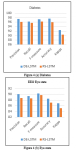
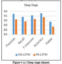
Figure 4. Classification results analysis of DE-LSTM and RS-LSTM models (a) Diabetes, (b) EEG Eye State and (c) Sleep stage dataset.

Table 5: Comparison of Proposed DE-LSTM with State of Arts for Diabetes Datasets in terms of Accuracy

Classifiers	Accuracy (%)
DE-LSTM	97.59
DE-GRU	96.34
DE-RNN	92.43
RS-LSTM	95.89
SA-LSTM	95.48
GRU	91.54
RNN	86.87
LSTM	91.75
MLP	81.90

Table 5 and Figure 6 offer a comparative analysis of the proposed models on the applied diabetes dataset in terms of accuracy. The

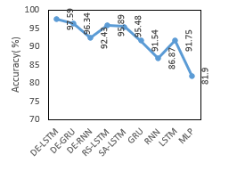
Figure 6. Accuracy analysis of various models on Diabetes Datasets

Table 6: Comparison of Proposed DE-LSTM with State of Arts for EEG Eye State in terms of Accuracy

Classifiers	Accuracy (%)
DE-LSTM	88.52
DE-GRU	87.14
DE-RNN	85.23
RS-LSTM	87.11
SA-LSTM	84.49
GRU	80.65
RNN	78.94
LSTM	81.78
Linear SVM	55.12
HMM	54.12

experimental values indicated that the RNN and MLP models have stated ineffective performance by attaining minimal accuracy values of 86.87% and 81.90% respectively. Next to that, the GRU and MLP models have reached to slightly higher and closer accuracy values of 91.54% and 91.75% respectively. Then, the DE-RNN model has accomplished better results with the accuracy of 92.43%. Simultaneously, the RS-LSTM and SA-LSTM models have accomplished manageable results with the closer accuracy values of 95.89% and 95.48% respectively. On continuing with, the near optimal accuracy of 96.34% has been offered by the DE-GRU model. However, the DE-LSTM model has outperformed all the compared methods with the maximum accuracy of 97.59%.

Table 6 and Figure 7 provide a comparative analysis of the presented models on the applied EEG Eye State with respect to accuracy. The experimental values implied that the Linear SVM as well as HMM methods have shown inferior function by reaching lower and same accuracy values of 55.12%. Then, the RNN and GRU models have attained better and nearby accuracy values of 78.94% and 80.65% correspondingly. Followed by, the LSTM and SA-LSTM approaches have achieved manageable accuracy values of 81.78% and 84.49% respectively. At the same time, the DE-RNN and RS-LSTM models have obtained considerable results with the nearby accuracy values of 85.23% and 87.11% correspondingly. Along with that, the near optimal accuracy of 87.14% is provided by the DE-GRU model. Thus, the DE-LSTM model has performed well than other approaches with the higher accuracy of 88.52%.

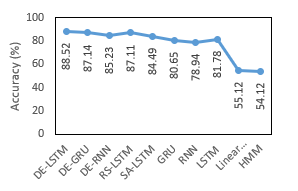
Figure 7: Accuracy analysis of various models on EEG Eye State

Table 7: Comparison of Proposed DE-LSTM with State of Arts for Sleep Stage Dataset in terms of Accuracy

Classifiers	Accuracy (%)
DE-LSTM	93.18
DE-GRU	91.57
DE-RNN	87.93
RS-LSTM	91.49
GRU	85.42
RNN	82.19
LSTM	86.45
CNN	78.23
5C-CNN	83.20
7C-CNN	87.50
9C-CNN	89.00
11C-CNN	90.12
DBN	72.20
SAE	77.70
RBF	81.70

Figure 8: Accuracy analysis of various models on Sleep Stage Dataset

Table 7 and Figure 8 show a comparative analysis of the proposed method on the given Sleep Stage Dataset in terms of accuracy. The experimental values showcased that the DBN model has revealed poor performance by accomplishing lower accuracy values of 72.20%. Then, the SAE, CNN and RBF models have attained reasonable performance and closer accuracy values of 77.70%, 78.23% and 81.70% respectively. Next to that, the RNN, 5C-CNN and GRU methods have achieved appreciable results with the accuracy values of 82.19%, 83.20% and 85.42% respectively. Meantime, 7C-CNN, LSTM and DE-RNN frameworks have attained better results with the near accuracy values of 86.45%, 87.50% and 87.93% correspondingly. Concurrently, the 9C-CNN, 11C-CNN and RS-LSTM methodologies have performed better results with accuracy values of 89%, 90.12% and 91.49% respectively. In line with this, the closer and best accuracy of 91.57% has been provided by the DE-GRU model. Therefore, the DE-LSTM model functions an outstanding performance of related models with optimal accuracy of 93.18%. From the above mentioned tables and figures, it is evident that the proposed DE-LSTM model can be employed as an appropriate medical data classification model. Besides, it is ensured that the inclusion of hyper parameter tuning technique helps to improvise the classification performance.

8. Conclusion

This paper has presented a new hyperparameters tuned DL models for intelligent medical diagnosis and classification. The proposed model involves different processes namely pre-processing, feature extraction, classification, and parameter optimization. Initially, the input data is pre-processed to remove the unwanted data and transform it to a compatible format. Then, SA-FS process takes place to select the useful subset of features. Then, DL models are applied to carry out the classification process. Finally, DE is applied for the parameter optimization of the DL models. A detailed simulation analysis takes place using three benchmark medical dataset namely Diabetes, EEG Eye State and Sleep stage dataset. The simulation outcome indicated that the DE-LSTM model have shown better performance with the maximum accuracy of 97.59%, 88.52% and 93.18% on the applied diabetes, EEG Eye State and Sleep stage dataset. In future, the performance of the proposed models can be improved by the use of clustering techniques and learning rate scheduler.

Conflict of Interest

The authors declare no conflict of interest.

1. A. Gottlieb, G.Y. Stein, E. Ruppin, R.B. Altman, R. Sharan, “A method for inferring medical diagnoses from patient similarities,” BMC Medicine, 11, 194, 2013, doi:10.1186/1741-7015-11-194.
2. R. Miotto, F. Wang, S. Wang, X. Jiang, J.T. Dudley, “Deep learning for healthcare: Review, opportunities and challenges,” Briefings in Bioinformatics, 19(6), 1236-1246, 2017, doi:10.1093/bib/bbx044.
3. I. Tobore, J. Li, L. Yuhang, Y. Al-Handarish, A. Kandwal, Z. Nie, L. Wang, “Deep learning intervention for health care challenges: Some biomedical domain considerations,” Journal of Medical Internet Research, 7(8), e11966, 2019, doi:10.2196/11966.
4. R. Bellazzi, B. Zupan, “Predictive data mining in clinical medicine: Current issues and guidelines,” International Journal of Medical Informatics,77(2), 81-97, 2008, doi:10.1016/j.ijmedinf.2006.11.006.
5. G. LeCun, Y., Bengio, Y., Hinton, “Deep learning. Nature,” 521 (7553), 436–444, 2015, doi:10.1038/nature14539.
6. T. Young, D. Hazarika, S. Poria, E. Cambria, “ Recent trends in deep learning based natural language processing [Review Article], ” IEEE Computational Intelligence Magazine, 13(3), 55-75, 2018, doi:10.1109/MCI.2018.2840738.
7. J. Powles, H. Hodson, “Google DeepMind and healthcare in an age of algorithms,” Health and Technology, 7(4), 351-367, 2017, doi:10.1007/s12553-017-0179-1.
8. A. Qayyum, J. Qadir, M. Bilal, A. Al Fuqaha, “Secure and Robust Machine Learning for Healthcare: A Survey,” IEEE Reviews in Biomedical Engineering, 2020, doi:10.1109/RBME.2020.3013489.
9. Y. Cheng, F. Wang, P. Zhang, J. Hu, “Risk prediction with electronic health records: A deep learning approach,” in 16th SIAM International Conference on Data Mining, 432-440, 2016, doi:10.1137/1.9781 611974348.49.
10. T. Pham, T. Tran, D. Phung, S. Venkatesh, “Predicting healthcare trajectories from medical records: A deep learning approach,” Journal of Biomedical Informatics, 16, 218-229, 2017, doi:10.1016/j.jbi. 2017.04.001.
11. E. Choi, M.T. Bahadori, A. Schuetz, W.F. Stewart, J. Sun, “Doctor AI: Predicting Clinical Events via Recurrent Neural Networks.,” JMLR Workshop and Conference Proceedings, 301-318, 2016.
12. R. Miotto, L. Li, B.A. Kidd, J.T. Dudley, “Deep Patient: An Unsupervised Representation to Predict the Future of Patients from the Electronic Health Records,” Scientific Reports, 6(1), 1-10, 2016, doi:10.1038/srep26094.
13. Z. Liang, G. Zhang, J.X. Huang, Q.V. Hu, “Deep learning for healthcare decision making with EMRs,” in Proceedings IEEE International Conference on Bioinformatics and Biomedicine(BIBM),556-559, 2014, doi:10.1109/BIBM.2014.6999219.
14. Z.C. Lipton, D.C. Kale, C. Elkan, R. Wetzel, “Learning to diagnose with LSTM recurrent neural networks,” in 4th International Conference on Learning Representations, ICLR 2016 – Conference Track Proceedings, 2016.
15. Z. Che, D. Kale, W. Li, M.T. Bahadori, Y. Liu, “Deep computational phenotyping,” in Proceedings of the ACM SIGKDD International Conference on Knowledge Discovery and Data Mining, 507-516, 2015, doi:10.1145/2783258.2783365.
16. T.A. Lasko, J.C. Denny, M.A. Levy, “Computational Phenotype Discovery Using Unsupervised Feature Learning over Noisy, Sparse, and Irregular Clinical Data,” PLoS ONE, 8(6), e66341, 2013, doi:10.1371/journal.pone.0066341.
17. D. Kollias, A. Tagaris, A. Stafylopatis, S. Kollias, G. Tagaris, “Deep neural architectures for prediction in healthcare,” Complex & Intelligent Systems, 4(2),119-131, 2018, doi:10.1007/s40747-017-0064-6.
18. T. Tran, T.D. Nguyen, D. Phung, S. Venkatesh, “Learning vector representation of medical objects via EMR-driven nonnegative restricted Boltzmann machines (eNRBM),” Journal of Biomedical Informatics, 54, 96-105, 2015, doi:10.1016/j.jbi.2015.01.012.
19. P. Nguyen, T. Tran, N. Wickramasinghe, S. Venkatesh, “Deepr: A Convolutional Net for Medical Records,” IEEE Journal of Biomedical and Health Informatics, 21, 22-30, 2017, doi:10.1109/JBHI.2016. 2633963.
20. R. Panthong, A. Srivihok, “Wrapper Feature Subset Selection for Dimension Reduction Based on Ensemble Learning Algorithm,” in Procedia Computer Science, 72, 162-169, 2015, doi:10.1016/j.procs. 2015.12.117.
21. B. Nakisa, M.N. Rastgoo, A. Rakotonirainy, F. Maire, V. Chandran, “Long short term memory hyperparameter optimization for a neural network based emotion recognition framework,” IEEE Access, 6, 49325-49338, doi:10.1109/ACCESS.2018.2868361.

(Click Here)

(Click Here)