1. Introduction

This paper is an extension of work originally presented in the Proceedings of the EUROCON 2019 – 18th International Conference on Smart Technologies [1].

1.1. Wireless Sensor Networks

Wireless sensor networks (WSNs) are a technology formed by smallsize autonomous low-cost sensor nodes equipped with three basic components – a sensing subsystem, a processing subsystem, and a wireless communication subsystem [2]–[4]. These subsystems enable the sensor nodes to concurrently sense the surrounding area, to process the measured data, and to communicate with each other via wireless transmission channels [2, 3]. Moreover, the sensor nodes are supplied by an energy source, allowing WSNs to execute the programmed tasks [3]. WSNs are required to obtain a lot of information about the observed physical phenomenon (e.g., light, motion, temperature, seismic events, humidity, pressure, etc.) and to effectively deliver the measured data to the end-users [3, 5]. Furthermore, they are self-organizing systems typically consisting of many sensor nodes (i.e., hundreds or even thousands) distributed over large-scale areas (either in a random fashion or manually) whereby large geographical territories can be cooperatively monitored with very high precision [2, 6]. As WSNs are generally built-up on an ad-hoc basis, the deployment of the sensor nodes is significantly simplified [7]. In many applications, the sensor nodes are required to operate under inhospitable environmental conditions and without any human interaction; therefore, the design of the algorithms for WSNs has to be affected by these facts [2]. So, WSN-based applications have to be viable and energy-efficient so that the robustness of WSNs to potential threads is high [2]–[4]. Over the last years, WSNs have found the application in various areas such as industrial monitoring, health care, localization, security, structural monitoring, military monitoring, etc. [8].

1.2. Consensus-based Algorithms for Data Aggregation

As the sensor nodes are vulnerable to numerous threats (e.g., temperature, radiation, pressure variations, electromagnetic noise, coverage problems, a high failure rate, etc.) and can measure highly correlated or even duplicated information, complementary algorithms for data aggregation are applied in many WSN-based applications in order to suppress these negative factors and to optimize the overall energy consumption (see Figure 1 for an example demonstrating the difference between WSNs with and without data aggregation) [9, 10]. In addition, data aggregation algorithms can optimize also routing mechanisms, thereby reducing the total energy requirements as well [11]. In the literature, one can find several papers concerned with how to effectively bound algorithms for data aggregation whereby the communication, computation, and energy requirements of WSNs can be optimized [12]–[14]. Note that data aggregation is an important process not only in WSNs but also in other industries [15]–[18].

Over the last decades, consensus-based algorithms for data aggregation have significantly gained the attention of the worldwide scientific community [13, 17, 19]. The problem of consensus achievement poses one of the most fundamental challenges in distributed computing [20]. In WSNs, the term consensus, in general, means the task of getting a group of the sensor nodes to agree on a common value determined by the initial states of all the sensor nodes in this group [21]. The consensus is achieved either asymptotically or in a bounded time interval due to iterative mutual interactions among these sensor nodes [21]. Eventually, each sensor node knows the exact value or an estimate of the wanted aggregate function. Gutierrez-Gutierrez et al. [22] define two categories of consensus-based algorithms for data aggregation, namely the deterministic and the stochastic algorithms. In the literature, one can find many deterministic approaches, e.g., the Maximum Degree weights algorithm, the Metropolis-Hastings algorithm (MH), the Best Constant weights algorithms, the Convex Optimized weights algorithm, etc. [1, 13, 19]. Probably, the most frequently quoted stochastic consensus-based algorithms are the Push-Sum algorithm, the PushPull algorithm, the Broadcast gossip algorithm, the Pairwise gossip algorithm, the Geographic gossip algorithm, etc. [14, 22]–[25]. As stated in [4], the algorithms differ from each other in many aspects such as the convergence rate, the robustness to potential threats, the initial configuration, the performance in mobile systems, etc.

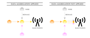
Figure 1: Comparison of WSN with/without data aggregation

1.3. Generalized Metropolis-Hastings for Data Aggregation

In this paper, we focus our attention on MH, which was proposed by

Nicolas Metropolis et al. in the 1950s and extended by Wilfred Keith Hastings approximately twenty years later [1]. Since its definition, it has found the application in various areas, e.g., simulating multivariate distributions, block-at-a-time scans, acceptance-rejection sampling, etc. [1]. Lately, Schwarz et al. have defined its generalized variant (referred to as the generalized Metropolis-Hastings algorithm and labeled as GMH) and derived the convergence conditions over arbitrary graphs including critical topologies such as bipartite regular graphs [26]. This algorithm poses a multi-functional distributed linear consensus algorithm able to estimate various aggregate functions, namely the arithmetic mean, the sum, and the graph order. Its weight matrix is symmetric and doubly stochastic, and each graph edge is allocated a weight determined by the degrees of two linked vertices [1]. Thus, this algorithm represents a fully-distributed approach in contrast to many other distributed consensus-based algorithms for data aggregation that require global information for the optimal initial configuration and the proper operating (e.g., the maximum degree, the Laplacian spectrum, etc.) [19]. Therefore, this algorithm (including its original version) has significantly attracted the attention of the world-wide scientific community over the past years [1].

1.4. Summary of Contribution

In this paper, we extend the analysis from [1], where GMH for distributed averaging with the stopping criterion proposed in [27] is analyzed. The extension presented in this paper lies in an analysis of GMH also for distributed summing and distributed graph order estimation. Thus, we compare GMH for estimating different aggregate functions with a various mixing parameter and under various initial configurations of the implemented stopping criterion over 100 unique random geometric graphs (RGGs). In [1], it is identified that GMH can be applied to estimate the arithmetic mean, which motivates us to examine and to compare the applicability of GMH to estimating also other aggregate functions. In the case of distributed summing, we carry out two scenarios – either the initial inner states or the final estimates (i.e., the inner states after the consensus is achieved) are multiplied by the graph order. Thus, the experimental section consists of four scenarios. Finally, GMH for distributed summing and distributed graph order estimation is compared to our previous work where the average consensus algorithm is analyzed

[8].

1.5. Paper Organization

The content of this paper is organized as follows:

• Section 1: is divided into five subsections:
  • Section 1.1: provides basic information about WSNs, i.e., a brief introduction about this technology, its purpose, constraints, and application.
  • Section 1.2: is concerned with consensus-based algorithms, i.e., a brief introduction into data aggregation/these algorithms, their purpose, classification, and examples.
  • Section 1.3: deals with GMH and introduces its history, application, purpose, and features.
  • Section 1.4: is focused on a summary of our contribution presented in this paper.
• Section 2: is concerned with a literature review focused on the application of GMH in (not only) WSNs.
• Section 3: provides a theoretical insight into the topic and is partitioned into two subsections:
  • Section 3.1: introduces the applied mathematical model of WSNs, the definition of GMH, its convergence conditions, and the analyzed functionalities of GMH.
  • Section 3.2: deals with the implemented stopping criterion, i.e., why to implement it, its parameters, and its principle.
• Section 4: is focused on the applied research methodology and the metrics for performance evaluation.
• Section 5: consists of the experimentally obtained results in Matlab2018b (32 figures in overall), an analysis of the depicted results, a comparison of various functionalities of GMH, and a comparison of GMH to the average consensus algorithm.
• Section 6: briefly summarizes the outcomes of the research presented in this paper.

2. Literature Review

In this section, we turn our attention to the applicability of MH for various purposes in (not only) WSNs.

In [29], the authors focus their attention on data acquisition in

WSNs. They apply MH to determine the mixing time, which is the minimal length of a random walk to approximate a uniform stationary distribution. In the next paper [30], the authors propose an approach for estimating the model parameters for time synchronization in WSNs. Here, they apply MH in combination with Gibbs samples for estimating the parameters of the Bayesian model. The paper [31] is concerned with the tuning parameters of WSNs. In this case, MH is used to determine the acceptance probability. For higher values of the temperature, the algorithm accepts all the moves, meanwhile, stochastic hill-climbing is performed in the case of lower temperatures. The authors of [32] apply a random walk as a routing scheme and compressive sensing to recover raw data in order to optimize the communication costs and detection performance. MH is used to choose neighbors that receive a message. In [33], a novel approach based on MH that synthesizes safe reversible Markov chains is introduced. The authors of [34] propose an approach for evaluating the network loss probability of the mobile collectors for harvesting data in WSNs. As stated in the paper, the optimal movement strategy is achieved in the case of applying MH. In [35], the authors provide a Markov point process model to generate evolving geometric graphs capable of responding to external effects. In the presented model, the vertices can move according to MH-based rules, giving a random pattern of points whose distribution is similar to the Markov point process distribution. In [36], MH finds an application to obtaining a sequence of random samples from an arbitrary distribution. The biggest benefit of applying MH is that this algorithm is independent of the normalization factor. In the paper [37], a novel MH-based algorithm assumed to protect WSNs from internal attacks is proposed and analyzed. In this approach, MH is used to generate the samples from a stationary distribution. In [38], the authors propose a spatialtemporal data gathering mechanism based on MH with delayed acceptance. This approach allows harvesting compressive data by sequentially visiting small subsets of nodes along a routing path. In [13], MH is analyzed over WSNs with embedded computing and communication devices. A centralized stopping criterion based on the mean square error is applied to bound the algorithm execution in this paper. The authors of [39] propose a novel consensus-based algorithm for data aggregation over WSNs by combining MH with the convex optimized weights algorithm, thereby optimizing both the transient and the steady-state algorithm phase. In [40], MH is applied to target tracking in WSNs for surveillance tasks. The proposed approach is to convert binary detections into finer position reports by applying the spatial correlation. The mechanism for a node-specific interference problem appearing in heterogeneous WSNs is proposed in [41]. In this approach, MH is employed in its first step. In [42], it is stated that MH can be used to choose the next nodes in random walks. The paper [43] is focused on a modified MH for estimating the item, structural, and Q matrix parameters. In [44], the authors propose a TunaMH method based on MH (as its name evokes) for exposing a tunable tradeoff between its batch size and the convergence rate that is theoretically guaranteed. The authors of [45] propose a novel MH to provide large proposal transitions accepted with a high probability due to a significant increase in the complexity and in the dimension of the interference problems. The authors of [46] address the incipient fault detection problem, which is solved by the proposed two-step technique. In the second step, MH is used to perform the change point detection. In [47], the authors present a received signal strength-based inter-network cooperative localization approach utilizing MH. At the end of this section, as mentioned above, Schwarz et al. define the generalized variant of MH and analyze its convergence in [26].

Thus, it can be seen that our contribution is an analysis of GMH for estimating three aggregation functions with the fully-distributed stopping criterion from [27]. In none of the provided papers, such a deep analysis of GMH for data aggregation with a stopping criterion proposed primarily for WSNs is carried out.

3. Theoretical Background

3.1. Model of GMH for Estimating Average/Sum/Graph Order in WSNs

In this paper, WSNs are modeled as undirected simple finite graphs

(with the graph order n) formed by two time-invariant sets, namely the vertex set V and the edge set E (G = (V, E)), and so the graph order and the graph size are constant [1]. The vertex set V gathers all the graph vertices, which represent the sensor nodes in WSN and are distinguishable from each other by the unique index number, i.e., V = {v_i : i = 1,2,…n}. The edge set E is formed by all the graph edges representing the direct connection between two vertices (v_i and v_j are linked by e_ij). Subsequently, the neighbor set of v_i, which is a set consisting of all the neighbors of the corresponding node, can be defined as follows [1]:

From a global view, GMH can be modeled as follows [26]:

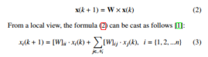
Here, x(k)^[1] is a variant column vector containing the inner states of all the sensor nodes in WSN at the corresponding iteration, and W is the weight matrix defined for GMH as follows [26]:

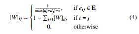
Here, d_i poses the degree of v_i, and  represents the mixing parameter, which has to take a value from the following interval for the convergence achievement [26]:

Note that the convergence is obtained for  = 0 only unless the underlying graph is bipartite regular [26]. As stated in [26], the adjacency matrix A of a bipartite graph has a block structure with zero diagonal in the case of  = 0, which implies:

Thus, the sensor nodes are divided into two groups, and their inner states oscillate between two values equal to the arithmetic means determined by the inner states of the sensors nodes in these groups. The mixing parameter  = 0 causes the equality in ρ(L_e)² ≤ 2 in the case of the bipartite regular graphs, resulting in the divergence of the algorithm:

n

In Figure 14, we show the evolution of the inner states over a random bipartite regular graph for four values of the mixing parameter , including  = 0. From the figures, it can be seen that the inner states converge to the arithmetic mean except for  = 0, when the algorithm diverges.

Properly configured GMH operates in such a way that the inner state of each sensor node asymptotically converge to the value of the estimated aggregated function (which determines the value of the steady-state), i.e. [1]:

1

Here, 1 poses an all-ones vector formed by n elements, and 1^T is its transpose. In the following part, examples of how the inner states evolve with an increase in the iteration number for each analyzed functionality of GMH are shown.

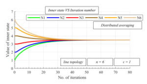
Figure 2: Inner states as function of number of iterations over line topology with graph order n = 6 – distributed averaging, mixing parameter  = 1

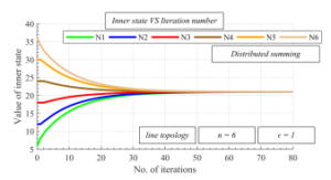
Figure 3: Inner states as function of number of iterations over line topology with graph order n = 6 – distributed summing, mixing parameter  = 1

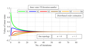
Figure 4: Inner states as function of number of iterations over line topology with graph order n = 6 – distributed graph order estimation, mixing parameter  = 1

The existence of the limit (8) is essential for GMH to operate correctly and is ensured, provided that these three convergence conditions are met [26]:

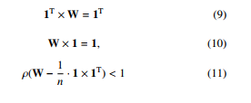
n

Here, ρ(·) is the spectral radius of the corresponding vector/matrix, and its value is equal to the largest eigenvalue in the absolute value from the corresponding spectrum, i.e.:

Here, λ_i(·) is the i^th largest eigenvalue from the corresponding spectrum.

As mentioned earlier, GMH can estimate three various aggregate functions, namely the arithmetic mean, the sum, and the graph order. The values of the initial inner states are affected by the estimated aggregate function as follows:

• Distributed averaging: the initial inner states are equal to (for example) independent local measurements.
• Distributed summing: the initial inner states are equal to (for example) independent local measurements and multiplied by the graph order n – this multiplication is carried out either before the algorithm begins or after completing the algorithm.
• Distributed graph order estimation: one of the sensor nodes is selected as the leader, and its initial inner state is equal to

”1”. The other sensor nodes initiate their inner state with ”0”. Once the consensus is achieved, the sensor nodes determine the inverted value from the final estimates, which is equal to an estimate of the graph order n.

3.2. Distributed Stopping Criterion for WSNs

In this section, we introduce the implemented stopping criterion for bounding the execution of GMH. As mentioned earlier, an effectively stopped execution may significantly optimize the algorithm in terms of many aspects such as the overall energy consumption, the communication amount, etc., and therefore, a proper initial configuration of the implemented stopping criterion is essential especially in energy-constrained technologies such as WSNs. In this paper, we analyze the fully-distributed stopping criterion from [27], which is determined by two constants:

• accuracy
• counter threshold

Algorithm 1 GMH for distributed averaging/summing/graph order estimation with bounded execution At the beginning of the algorithm (i.e., k = 0), every sensor node vi ∈ V initiates its inner state (i.e., xi(0)) with a scalar value according to the estimated aggregate function: •    Distributed averaging: the initial inner states are equal to (for example) independent local measurements. •    Distributed summing: the initial inner states are equal to (for example) independent local measurements and multiplied by the graph order n – this multiplication is carried out either before the algorithm begins or after completing the algorithm. •    Distributed graph order estimation: one of the sensor nodes is selected as the leader, and its initial inner state is equal to ”1”. The other sensor nodes initiate their inner state with ”0”. Once the consensus is achieved, the sensor nodes determine the inverted value from the final estimates. Also, each sensor node vi ∈ V sets its counter to ”0”. The parameters counter threshold and accuracy are constant during the algorithm execution and set to the same value at each sensor node. Each sensor node is considered to be active until it locally completes the algorithm. . . . . . . . . . . . . . . . . . . . . . . . . . . . . . . . . . . . . . . . . . . . . . . . . . . . . . . . . . . . . . . . . . . . . . . . . . . . . . . . . . . . . . . . . . . . . . . . . . . . . . . . . . . . . . . . . . . . . . . . . . . . At the next iterations (i.e., k = 1, 2, …), every active sensor node repeats the following steps as long as it is active: 1.    sends a broadcast message containing its current inner state to (1) as well as collecting the inner states from (1). 2.    updates its inner state for the next iteration by applying the update rule (2)/(3). 3.    verifies whether the finite difference between two subsequent inner states is smaller than accuracy, i.e., |∆xi(k)| < accuracy. If it is true, it increments its counter by ”1”, otherwise, sets it to ”0”. 4.    verifies the condition: counter = counter threshold. If it is valid, the corresponding sensor node considers GMH to be locally completed, and this sensor node becomes inactive. If it is invalid, the sensor node repeats the previous steps.

Both constants are the same at each sensor node and have to be set before the algorithm begins. Also, each sensor node has its own counter, which is a variable initiated by ”0” at each sensor node. The principle of the stopping criterion lies in a comparison of the finite difference between two subsequent inner states at each sensor node with pre-set accuracy. If the finite difference is smaller than accuracy counter threshold-times in the array, the algorithm is locally completed at the corresponding nodes, and this node does not participate in the algorithm anymore. If not, the value of counter is reset regardless of its current state. See Algorithm 1 for the formalization of GMH with the stopping criterion from [27].

4. Research Methodology

This section is concerned with the applied research methodology and the metrics for performance evaluation.

As already mentioned in this paper, the weight matrix of GMH is modifiable by changing the value of the mixing parameter . As stated in [26], the convergence is ensured for  taking value from (5) unless the underlying graph is bipartite regular. As it is not too likely that WSNs are bipartite regular [26], we do not include them in the experimental section – GMH diverges over these topologies, which may significantly skew the presented results. Therefore, we separately analyze these critical topologies in Section 3.1. In the experimental section, the mixing parameter  takes the following four values:

• = {1, 2/3, 1/3, 0}

As mentioned above, we apply the stopping criterion from [27] to bound the algorithm. In our experiments, its configuration is selected as follows:

• accuracy = {10⁻², 10⁻⁴, 10⁻⁵, 10⁻⁶}
• counter threshold = {3, 5, 7, 10, 20, 40, 60, 80, 100}

As mentioned earlier, the performance of GMH with various initial configurations is tested over RGGs with the graph order n = 200 see Figure 5 for their representatives. For the sake of high research credibility, we generate 100 graphs each with a unique topology where the algorithm is examined.

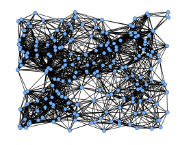
Figure 5: Representative of random geometric graphs

In the experimental part, we analyze GMH estimating three different aggregate functions, and therefore we partition the content of the experimental part into four scenarios as follows:

 Scenario 1 – GMH estimates the arithmetic mean from all the initial inner states, which are independent and identically distributed random values of the standard Gaussian distribution,

i.e.:

 Scenario 2 – the algorithm determines estimates of the sum calculated from all the initial inner states, which are IDD random values of the same distribution as in the previous scenario. The inner states are multiplied by the graph order n before GMH begins.

 Scenario 3 – in this scenario, GMH also estimates the sum from all the initial inner states like in Scenario 2, compared to which the inner states are multiplied by the graph order n after the consensus is achieved.

 Scenario 4 – the graph order n, i.e., the size of a network, is estimated in this scenario. One of the vertices is selected as the leader, whose initial inner state is equal to ”1”, meanwhile, the other ones initiate their initial inner state with ”0” (in our analyses, the best-connected node is the leader), i.e.:

The inverted value of the inner states is determined after the consensus is achieved.

To evaluate the performance of the algorithm, we apply two metrics:

• Mean Square Error (MSE): is used to quantify the precision of the final estimates and defined as follows [48, 49]:

Here, k_l is the iteration when the consensus is achieved.

• Convergence rate: quantifies the algorithm speed (labeled as k_l) and is expressed as the number of the iterations for the consensus achievement among all the sensor nodes in WSN.

In all the shown figures, we depict and analyze the average of both metrics over 100 graphs for each accuracy, counter threshold, and the mixing parameter .

5. Experimental Section

In this section, we provide and discuss numerical experiments executed in Matlab2018b. As mentioned above, we extend the analysis of bounded GMH from [1], where this algorithm for distributed averaging is analyzed in terms of the estimation precision and the convergence rate. In this work, the extension lies in an analysis of GMH for distributed summing (either the initial inner states or the final estimates are multiplied by the graph order n) and GMH for graph order estimation. Also, GMH is compared to the average consensus algorithm. The experimental section consists of:

Table 1: List of figures provided in experimental section

Figure	Applied Metric	Scenario	Note
No. 6	MSE	No. 1	Cited from [1]
No. 7	Convergence rate	No. 1	Cited from [1]
No. 8	MSE	No. 2
No. 9	Convergence rate	No. 2
No. 10	MSE	No. 3
No. 11	Convergence rate	No. 3
No. 12	MSE	No. 4
No. 13	Convergence rate	No. 4

The first part is concerned with an MSE analysis of all the functionalities of GMH. From Figure 6, Figure 8, Figure 10, and Figure 12, it is seen that an increase in counter threshold and a decrease in accuracy result in a decrease in MSE, whereby the precision of the final estimates is increased in each scenario. Also, lower values of the mixing parameter  ensure that the value of MSE is

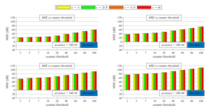
Figure 6: Estimation precision quantified by mean square error for various configurations of implemented stopping criterion and different mixing parameter – generalized Metropolis-Hastings for distributed averaging – Scenario 1

Figure 7: Convergence rate expressed as iteration number required for consensus achievement for various configurations of implemented stopping criterion and di mixing parameter – generalized Metropolis-Hastings for distributed averaging – Scenario 1

lower regardless of the estimated aggregate function. Furthermore, we can see that the algorithm achieves the highest precision in the case of estimating the graph order (i.e., in Scenario 4). The values of MSE, in this case, are from the range [−110.7, −43.2]³. The second highest precision is obtained when the arithmetic mean is estimated (Scenario 1). In this case, the values of MSE are from

the range [−110.4, −20.88]³. The worst estimation precision is observed in the case of sum estimation. Here, Scenario 2 (MSE is from [−109.9,4.288]³) outperforms Scenario 3 (MSE is from [−64.36,25.14]³), proving that multiplying the initial inner states with the graph order n ensures higher precision of the algorithm than multiplying the final estimates. As mentioned earlier, we analyze the average consensus algorithm for distributed summing and dis-

Figure 8: Estimation precision quantified by mean square error for various configurations of implemented stopping criterion and different mixing parameter – generalized Metropolis-Hastings for distributed summing – Scenario 2

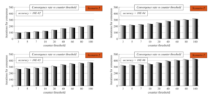
Figure 9: Convergence rate expressed as iteration number required for consensus achievement for various configurations of implemented stopping criterion and di mixing parameter – generalized Metropolis-Hastings for distributed summing – Scenario 2

tributed graph order estimation in our previous work [8]. Compared to those results, it can be seen that GMH outperforms the average consensus algorithms for estimating both examined aggregate functions. For counter threshold = 100, accuracy = 10⁻⁶, and  ensuring the highest performance, GMH outperforms the average consensus algorithm by 12.78 dB in Scenario 2, by 77.31 dB in Scenario 3, and by 104.469 dB in Scenario 4. Moreover, an important fact

identified in [8] is that the average consensus achieves a very low estimation precision for lower values of counter threshold and higher values of accuracy in the case of graph order estimation, making the algorithm unusable with these configurations of the stopping criterion. However, in this paper, we identify that this phenomenon is not visible in the case of GMH; therefore, this algorithm is much more appropriate for graph order estimation than the average con-

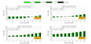
Figure 10: Estimation precision quantified by mean square error for various configurations of implemented stopping criterion and different mixing parameter – generalized Metropolis-Hastings for distributed summing – Scenario 3

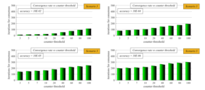
Figure 11: Convergence rate expressed as iteration number required for consensus achievement for various configurations of implemented stopping criterion and di mixing parameter – generalized Metropolis-Hastings for distributed summing – Scenario 3

sensus algorithm when the stopping criterion [27] is implemented. In addition, the value of the mixing parameter  has a less intensive impact on MSE compared to the average consensus algorithm for distributed summing/distributed graph order estimation. In the following part, we turn our attention to the convergence rate of GMH expressed as the iteration number for the consensus achievement. From Figure 7, Figure 9, Figure 11, and Figure 13, we can

see that an increase in counter threshold and a decrease in accuracy result in an increase in the number of the iterations required for the consensus; therefore, the convergence rate is decreased in each analyzed scenario. Again, a higher convergence rate in each scenario is obtained for lower values of the mixing parameter . Like in the previous analysis, Scenario 4 outperforms all three other scenarios also in terms of the convergence rate, and the convergence rate in this scenario is from the interval [5,240.5]³. As furthermore seen, the second-highest convergence rate is achieved by both Scenario 1 and Scenario 3 ([11.55,295.80]³); therefore, the number of the iterations for the consensus achievement is the same (with a few exceptions) in both scenarios. In contrast to the previous analysis, Scenario 2 ([95.78,420.9]³) is outperformed by Scenario 3, meaning that multiplying the final estimates ensures a higher convergence rate than multiplying the initial inner states. Compared to our pre-

Figure 12: Estimation precision quantified by mean square error for various configurations of implemented stopping criterion and different mixing parameter – generalized Metropolis-Hastings for distributed graph order estimation – Scenario 4

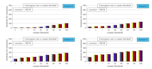
Figure 13: Convergence rate expressed as iteration number required for consensus achievement for various configurations of implemented stopping criterion and di mixing parameter – generalized Metropolis-Hastings for distributed graph order estimation – Scenario 4

vious work, GMH outperforms the average consensus algorithm also in terms of the convergence rate in both distributed summing and distributed graph order estimation. For counter threshold = 100, accuracy = 10⁻⁶, and  ensuring the highest performance, the convergence rate of GMH is greater than the convergence rate of the average consensus algorithm by 139.5 iterations in Scenario 2, by 87.3 iterations in Scenario 3, and by 52.5 iterations in Scenario 4. Also, like in the previous analysis, the value of the mixing parameter  has only a marginal impact on the convergence rate in contrast to the average consensus algorithm examined in [8].

6. Conclusion

In this paper, we provide an extension of the analysis of GMH for distributed averaging over WSNs published in the conference proceedings of IEEE Eurocon 2019. The extension presented in this paper lies in an analysis of GMH for estimating also other aggregate functions, i.e., distributed summing and distributed graph order estimation. In our analyses, the algorithm with a different mixing parameter  is bounded by a distributed stopping criterion with varied initial configurations (i.e., counter threshold takes the values (10⁻², 10⁻⁴, 10⁻⁵, 10⁻⁶), and accuracy takes the values (3, 5, 7, 10, 20, 40, 60, 80, 100)). The experimental part consists of four scenarios (i.e., these functionalities are analyzed: distributed averaging, distributed summing – the initial inner states are multiplied by the graph order n, distributed summing – the final estimates are multiplied by the graph order n, a distributed graph order estimation). From the presented results, it is seen that an increase in counter threshold and a decrease in accuracy result in higher precision of the algorithm, however, the convergence rate expressed as the iteration number of the consensus achievement is decreased as a consequence. Thus, regardless of the estimated aggregate function, the highest precision of the final estimates and the lowest convergence rate is ensured for the configuration accuracy = 10⁻⁶ and counter threshold = 100, and vice versa the configuration accuracy = 10⁻² and counter threshold = 3 results in the highest convergence rate and the lowest precision. Also, we identify that the optimal performance in terms of the estimation precision and the convergence rate is achieved for  = 0 (i.e., the lower bound of the mixing parameter ), and an increase in  causes lower precision and lower convergence rate. However, the value of the mixing parameter  does not have an essential impact on the algorithm performance according to both applied metrics. In the experimental section, also the performances of GMH for estimating the arithmetic mean, the sum, and the graph order are compared to each other. The best performance is achieved in the case of graph order estimation in terms of both the estimation precision and the convergence rate (for  = 0, the values of MSE lie in [−43.2, −110.7], and the convergence rate in [5,240.5]). The second-best performance is achieved when the arithmetic mean is estimated (for  = 0, MSE is from [−20.88, −110.4], and the convergence rate from [11.55,295.8]). Thus, the lowest precision and convergence rate are achieved in the case of sum estimation. Here, multiplying the initial inner states instead of the final estimates ensures higher precision of the algorithm (for  = 0, MSE [−109.9,4.29], the convergence rate [95.78,420.9]), meanwhile, multiplying the final estimates results in a higher convergence rate (for  = 0, MSE [−64.36,25.14], the convergence rate [11.55,295.8]). The most important fact identified in this paper is that GMH achieves a high estimation precision regardless of the estimated aggregation function; therefore, this research identifies its applicability to estimating also two other aggregate functions in WSNs. In addition, we also compare GMH for distributed summing and distributed graph order estimation to the average consensus algorithm, thereby identifying that GMH is more appropriate for data aggregation over WSNs with the implemented stopping criterion than the average consensus algorithm in both applied metrics – the estimation precision and the convergence rate expressed as the iteration number necessary for the consensus achievement. GMH outperforms the average consensus (in the case that the performances of the most precise configurations are compared) by 12.78 dB and 139.5 iterations in Scenario 2, by 77.31 dB and 87.3 iterations in Scenario 3, and by 104.469 and 52.5 iterations in Scenario 4.

Thus, the final conclusion of the presented research is that the lower bound of mixing parameter  ensures the highest performance in both the estimation precision and the convergence rate – so, in real-world implementations,  = 0 is recommended for use. Also, an increase in counter threshold and a decrease in accuracy cause the algorithm to be more precise but, on the other hand, decelerated regardless of the estimated aggregate function, meaning that the initial configuration of the stopping criterion has to be affected by the fact whether a WSN-based application requires more precise or faster data aggregation. The most important identified fact is that GMH is applicable to estimating all three examined aggregate functions in WSNs.

Conflict of Interest

The authors declare no conflict of interest.

Acknowledgment

This work was supported by the VEGA agency under the contract No. 2/0155/19 and by COST: Improving Applicability of Nature-Inspired Optimisation by Joining Theory and Practice (ImAppNIO) CA 15140. Since 2019, Martin Kenyeres has been a holder of the Stefan Schwarz Supporting Fund.

Appendix

Figure 14: Evolution of inner states over bipartite regular graph for four values of mixing parameter

Table 2: Tables summarizing presented experimental results

Maximal and minimal precision of GMH quantified by MSE

Scenario 1

Scenario 2

Scenario 3

Scenario 4

Max

Min

Max

Min

Max

Min

Max

Min

= 1

-108.7 dB

-20.69 dB

-108.3 dB

4.89 dB

-62.68 dB

25.33 dB

-109.1 dB

-43.03 dB

= 2/3

-109.2 dB

-20.73 dB

-108.8 dB

4.68 dB

-63.22 dB

25.29 dB

-109.6 dB

-43.08 dB

= 1/3

-109.8 dB

-20.8 dB

-109.4 dB

4.52 dB

-63.78 dB

25.22 dB

-110.2 dB

-43.14 dB

= 0

-110.4 dB

-20.88 dB

-109.9 dB

4.29 dB

-64.36 dB

25.14 dB

-110.7 dB

-43.2 dB

Maximal and minimal convergence rate of GMH quantified by iteration number

Scenario 1

Scenario 2

Scenario 3

Scenario 4

Max

Min

Max

Min

Max

Min

Max

Min

= 1

11.66 ite.

302.8 ite.

100.2 ite.

433.6 ite.

11.66 ite.

302.8 ite.

5.13 ite.

246 ite.

= 2/3

11.61 ite.

300.5 ite.

99.87 ite.

429.6 ite.

11.61 ite.

300.5 ite.

5.09 ite.

244.5 ite.

= 1/3

11.57 ite.

298.1 ite.

96.68 ite.

425.4 ite.

11.57 ite.

298.1 ite.

5.02 ite.

242.5 ite.

= 0

11.55 ite.

295.8 ite.

95.78 ite.

420.9 ite.

11.55 ite.

295.8 ite.

5 ite.

240.5 ite.

[1] Here, k is the label of an iteration, and x(k = 0) represents the initial inner states ²L_e is the weighted Laplacian matrix

1. M. Kenyeres, J. Kenyeres, “Applicability of Generalized Metropolis- Hastings Algorithm in Wireless Sensor Networks,” in 18th Interna- tional Conference on Smart Technologies (EUROCON 2019), 1–5, 2019, doi:10.1109/EUROCON.2019.8861554.
2. A. Al-Karaki, A. E. Kamal, “Routing Techniques in Wireless Sensor networks: A Survey,” Secur. Netw, 11(6), 6–28, 2004, doi:10.1109/MWC.2004.1368893.
3. G. Anastasi, M. Conti, M. Di Francesco, A. Passarella, “Energy conservation in wireless sensor networks: A survey,” Ad Hoc Netw., 7(3), 537–568, 2009, doi:10.1016/j.adhoc.2008.06.003.
4. M. Kenyeres, J. Kenyeres, “Average Consensus over Mobile Wireless Sensor Networks: Weight Matrix Guaranteeing Convergence without Reconfiguration of Edge Weights,” Sensors, 20(13), 3677, 2020, doi:10.3390/s20133677.
5. M. A. Mahmood, W. K. G. Seah, I. Welch, “Reliability in wireless sensor networks: A survey and challenges ahead,” Comput. Netw., 79, 166–187, 2015, doi:10.1016/j.comnet.2014.12.016.
6. W. Ye, J. Heidemann, D. Estrin, “An energy-efficient MAC protocol for wireless sensor networks,” in 21st Annual Joint Conference of the IEEE-Computer-and- Communications-Societies Location (INFOCOM 2002), 1567–1576, 2002, doi:10.1109 19408.
7. B. Rashid, M. H. Rehmani, “Applications of wireless sensor networks for urban areas: A survey,” J. Netw. Comput. Appl., 60, 192–219, 2016, doi:10.1016/j.jnca.2015.09.008.
8. M. Kenyeres, J. Kenyeres, “Distributed Network Size Estimation Executed by Average Consensus Bounded by Stopping Criterion for Wireless Sensor Networks,” in 24th International Conference on Applied Electronics (AE 2019), 1–6, 2019, doi: 10.23919/AE.2019.8867009.
9. D. Izadi, J. H. Abawajy, S. Ghanavati, T. Herawan, “A data fusion method in wireless sensor networks,” Sensors, 15(2), 2964–2979, 2015, doi:10.3390/s150202964.
10. B. Yu, J. Li, Y. Li, T. Herawan, “Distributed data aggregation scheduling in wire- less sensor networks,” in 28th Conference on Computer Communications (IEEE INFOCOM 2009), 2159–2167, 2009, doi:10.1109/INFCOM.2009.5062140.
11. L. Krishnamachari, D. Estrin, S. Wicker, “The impact of data aggrega- tion in wireless sensor networks,” in 22nd International Conference on Dis- tributed Computing Systems Workshops (ICDCSW 2002), 575–578, 2002, doi:10.1109/ICDCSW.2002.1030829.
12. N. Al-Nakhala, R. Riley, T. Elfouly, “Distributed algorithms in wireless sen- sor networks: An approach for applying binary consensus in a real testbed,” Comput. Netw., 79(14), 30–38, 2015, doi:10.1016/j.comnet.2014.12.011.
13. G. Stamatescu, I. Stamatescu, D. Popescu, “Consensus-based data aggregation for wireless sensor networks,” Control. Eng. Appl. Inf., 19(2), 43–50, 2017, doi:10.1016/j.comnet.2014.12.011.
14. D. Kempe, A. Dobra, J. Gehrke, “Gossip-based computation of aggregate information,” in 44th Annual IEEE Symposium on Foundations of Computer Science (FOCS 2003), 482–491, 2003.
15. K. Kenda, B. Kazic, E. Novak, D. Mladenic, “Streaming data fusion for the internet of things,” Sensors, 19(8), 1955, 2019, doi:10.3390/s19081955.
16. G. B. Markovic, V. S. Sokolovic, M. L. Dukic, “Distributed hybrid two-stage multi-sensor fusion for cooperative modulation classification in large-scale wireless sensor networks,” Sensors, 19(19), 4339, 2019, doi:10.3390/s19194339.
17. D. Merezeanu, M. Nicolae, “Consensus control of discrete-time multiagent systems,” U. Politeh. Buch. Ser. A, 79(1), 167–174, 2017.
18. V. Oujezsky, D. Chapcak, T. Horvath, P. Munster, “Security testing of active optical network devices,” in 42nd International Conference on Telecommunications and Signal Processing (TSP 2019), 9–13, 2019 doi:10.1109/TSP.2019.8768811.
19. L. Xiao, S. Boyd, “Fast linear iterations for distributed averaging,” Syst. Con- trol. Lett., 53(1), 65–78, 2004, doi:10.1016/j.sysconle.2004.02.022.
20. M. J. Fischer, N. A. Lynch, M. S. Paterson, “Impossibility of Distributed Consensus with One Faulty Process,” J. ACM, 32(2), 374–382, 1985, doi:10.1145/3149.214121.
21. Y. Zheng, Y. Zhu, L. Wang, “Consensus of heterogeneous multi-agent sys- tems,” IET Control. Theory Appl., 5(16), 1881–1888, 2011, doi:10.1049/iet- cta.2011.0033.
22. J. Gutierrez-Gutierrez, M. Zarraga-Rodriguez, X. Insausti, “Analysis of known linear distributed average consensus algorithms on cycles and paths,” Sensors, 18(4), 968, 2018, doi:10.3390/s18040968.
23. S. S. Kia, B. Van Scoy, J. Cortes, R. A. Freeman, K. M. Lynch, S. Mar- tinez, “Tutorial on Dynamic Average Consensus: The Problem, Its Ap- plications, and the Algorithms,” IEEE Control Syst., 39(3), 40–72, 2019, doi:10.1109/MCS.2019.2900783.
24. T. C. Aysal, M. E. Yildiz, A. D. Sarwate, A. Scaglione, “Broadcast gos- sip algorithms for consensus,” IEEE Control Syst., 57(7), 2748–2761, 2009, doi:10.1109/TSP.2009.2016247.
25. J. C. S. Cardoso, C. Baquero, P. S. Almeida, “Probabilistic estimation of network size and diameter,” in 2009 4th Latin-American Symposium on De- pendable Computing (LADC 2009), 33–40, 2009, doi:10.1109/LADC.2009.19.
26. V. Schwarz, G. Hannak, G. Matz, “On the convergence of average consen- sus with generalized metropolis-hasting weights,” in 2014 IEEE International Conference on Acoustics, Speech, and Signal Processing (ICASSP 2014), 5442–5446, 2014, doi:10.1109/ICASSP.2014.6854643.
27. Kenyeres, M. Kenyeres, M. Rupp, P. Farkas, “WSN implementation of the average consensus algorithm,” in 17th European Wireless Conference 2011 (EW 2011), 139–146, 2011.
28. M. Sartipi, R. Fletcher, “Energy-efficient data acquisition in wireless sensor networks using compressed sensing,” in 2011 Data Compression Conference (DCC 2011), 223–232, 2011, doi:10.1109/DCC.2011.29.
29. A.Chatterjee, P. Venkateswaran, “An efficient statistical approach for time synchronization in wireless sensor networks,” Int. J. Commun. Syst., 29(4), 722–733, 2016, doi:10.1002/dac.2944.
30. A. Munir, A. Gordon-Ross, S. Lysecky, R. Lysecky, “Online algorithms for wireless sensor networks dynamic optimization,” in 2012 IEEE Consumer Communications and Networking Conference (CCNC’2012), 180–187, 2012, doi: 10.1109/CCNC.2012.6181082.
31. M. Nguyen, Q. Cheng, “Efficient data routing for fusion in wireless sensor networks,” Signal, 1000(8), 11–15, 2012.
32. M. El Chamie, B. Ac¸ıkmes¸e, “Safe Metropolis-Hastings algorithm and its application to swarm control,” Syst. Control. Lett., 111, 40–48, 2018, doi:10.1016/j.sysconle.2017.10.006.
33. A. Vijayalakshmi, V. Bhuvaneswari, “Mobile agent based optimal data gathering in Wireless Sensor Networks,” in 10th International Confer- ence on Intelligent Systems and Control (ISCO 2016), 1–4, 2016, doi:10.1109/ISCO.2016.7726974.
34. D. J. Irons, J. Jordan, “Geometric networks based on Markov point processes with applications to mobile sensor networks,” in 2013 2nd International Con- ference on Mechanical Engineering, Industrial Electronics and Informatization (MEIEI 2013), 1–17, 2013.
35. N. Ramakrishnan, N. Ertin, R. L. Moses, “Assumed density filtering for learn- ing Gaussian process models,” in 2011 IEEE Statistical Signal Processing Workshop (SSP 2011), 257–260, 2011, doi:10.1109/SSP.2011.5967674.
36. M. R. Ahmed, H. Cui, X. Huang, “Smart integration of cloud computing and MCMC based secured WSN to monitor environment,” in 2014 4th International Conference on Wireless Communications, Vehicular Technology, Information Theory and Aerospace and Electronic Systems (VITAE 2014), 1–5, 2014, doi:10.1109/VITAE.2014.6934449.
37. H. Zheng, J. Li, X. Feng, W. Guo, Z. Chen, N. Xiong, “Spatial-temporal data collection with compressive sensing in mobile sensor networks,” Appl. Soft Comput., 17(11), 2575, 2017, doi:10.3390/s17112575.
38. V. Schwarz, G. Matz, “Nonlinear average consensus based on weight morphing,” in 2012 IEEE International Conference on Acoustics, Speech, and Signal Processing (ICASSP 2012), 3129–3132, 2012, doi:10.1109/ICASS.2012.6288578.
39. S. Oh, P. Chen, M. Manzo, S. Sastry, “Instrumenting wireless sensor networks for real-time surveillance,” in 2006 IEEE International Con- ference on Robotics and Automation (ICRA 2006), 3128–3133, 2006, doi:10.1109/ROBOT.2006.1642177.
40. L. Martino, J. Plata-Chaves, F. Louzada, “A Monte Carlo scheme for node- specific inference over wireless sensor networks,” in 2016 IEEE Sensor Ar- ray and Multichannel Signal Processing Workshop (SAM 2016), 1–5, 2016, doi:10.1109/SAM.2016.7569731.
41. M. T. Nguyen, K. A. Teague, “Compressive sensing based random walk routing in wireless sensor networks,” Ad Hoc Netw., 54, 99–110, 2017, doi:10.1016/j.adhoc.2016.10.009.
42. C. W. Liu, B. Andersson, A. Skrondal, “A Constrained Metropolis–Hastings Robbins–Monro Algorithm for Q Matrix Estimation in DINA Models,” Psy- chometrika, 85(2), 322-357, 2020, doi:10.1007/s11336-020-09707-4.
43. R. Zhang, A. F. Cooper, C. De Sa, “Asymptotically Optimal Exact Minibatch Metropolis-Hastings,” arXiv preprint arXiv:2006.11677, 2020.
44. Y. Marnissi, E. Chouzenoux, A. Benazza-Benyahia, J. C. Pesquet, “Majorize- Minimize Adapted Metropolis-Hastings Algorithm,” IEEE Trans. Signal Pro- cess., 68, 2356–2369, 2020, doi:10.1109/TSP.2020.2983150.
45. M. F. D’Angelo, R. M. Palhares, R. H. Takahashi, R. H. Loschi, L. M. Baccarini, W. M. Caminhas, “Incipient fault detection in induction machine stator-winding using a fuzzy-Bayesian change point detection approach,” Appl. Soft Comput., 11(1), 179–192, 2011, doi:10.1016
46. S. B¨uy¨ukc¸orak, G. K. Kurt, A. Yongac¸oglu, “Inter-network cooperative localiza- tion in heterogeneous networks with unknown transmit power,” in 28th Annual IEEE International Symposium on Personal, Indoor and Mobile Radio Com- munications (PIMRC 2017), 1–5, 2017, doi:10.1109/PIMRC.2017.8292505.
47. V. Skorpil, J. Stastny, “Back-propagation and K-means algorithms comparison,” in 8th International Conference on Signal Processing (ICSP 2006), 1871–1874, 2006, doi:10.1109/ICOSP.2006.345838.
48. S. S. Pereira, A. Pages-Zamora, “Mean square convergence of consensus algorithms in rando WSNs,” IEEE Trans. Signal Processs, 58(5), 2866–2874, 2010, doi:10.1109 3140.

(Click Here)

(Click Here)