1. Introduction

Based on the Presidential Regulation of the Republic of Indonesia Number 131 the year 2015 concerning the Determination of Disadvantaged Regions in 2015-2019, East Java Province is one of the 21 Provinces that are lagging in Indonesia. Not only that, but East Java Province is also the only Province in Java which has several disadvantaged district or city. Therefore, a study needs to be carried out to evaluate various problems of development inequality that have left some regions in East Java behind.
Government Regulation number 78 of the year 2014 article 6 paragraph 1 states that the determination of disadvantaged regions is carried out every 5 years based on criteria and indicators established by the Ministry of Villages, Development of Disadvantaged Regions, and Transmigration. In this case, the last disadvantaged region was determined in 2015 listed in Presidential Regulation number 131 of the year 2015 and will be re-established in 2020. In this study, the criteria used are survey data in 2014 and 2018, which sources data were obtained from the Central Statistics Agency in the form of data on village potential, statistics on people’s welfare and the profile of each province in a certain number of years. The data in 2014 are used as a comparison with government decisions related to the determination of disadvantaged regions in 2015. While the data in 2018 will be used as predictions for the determination of disadvantaged regions in 2020. The results of this study are expected to provide a relevant picture in which regions have the potential to be left behind in the future. Thus, the government of District/City can take policies towards their regions that are adjusted to the characteristics of each region to alleviate the region from being left behind.
In practice, the government determines disadvantaged regions based on Presidential Regulation Number 131 the Year 2015 Article 6 Paragraph 2, using composite aspects and range values. Statistically, the two methods are only suitable for analyzing numerical data. While in reality, indicators to determine the status of disadvantaged regions do not only refer to numerical data. But several indicators are categorical. Thus, if the composite aspect and interval values are used as an analysis, it will not be able to accommodate 6 criteria consisting of 33 indicators. To overcome this, a special method is needed that can accommodate all types of data, both categorical and numerical. The statistical method that can be used for clustering mixed data is the ensemble method [1]-[3]. In this study, the ensemble method used is Robust Clustering Using Link (ROCK). Ensemble ROCK method is a clustering method that uses the concept of distance to measure the similarity or closeness between a pair of data points [4], [5]. The advantage of the ensemble ROCK method is it has better accuracy compared to the agglomerative hierarchy method with good scalability [6].
Ensemble ROCK method has proven to be optimal for conducting mixed data clustering in solving various cases [7], such as the research conducted by Shashi Sharma and Ram Lal Yadav, the research proved that ensemble ROCK method is more optimal when compared to the K-Means method for the cluster analysis process [8]. Similar to the research conducted by Dwi Harid Setiadi, in the application of ensemble ROCK method for mapping disadvantaged regions, it proved to be more optimal when compared to the SWFM ensemble method [9]. Then Alvionita compared the SWFM and ROCK methods for grouping orange accessions. In that study, it was found that the ROCK method had better grouping performance than the SWFM method [10]. Therefore, in this study, researchers will evaluate disadvantaged regions in East Java based-on indicators Ministry of Villages, Development of Disadvantaged Regions, and Transmigration using ensemble ROCK method.

Related Works

In the last few years evaluation of disadvantaged regions has been carried out, including Anik Djuridah in his research evaluating the status of disadvantaged regions using Discriminant analysis [11]. In that research, it was only determined the number of indicators that influence the determination of the status of being left behind from an area, without being known with certainty which regions are included in the group of disadvantaged regions and not. Similar to the research conducted by Satria, Herman, and Fajar who analyzed the development of disadvantaged regions in East Java using Location Quotient dan Shift Share Esteban Marquillas analysis [12]. In that study, it was only used the GRDP (Gross Regional Domestic Product) variable.
Furthermore, Dwi Hariadi Setiadi in his final project was mapping the District/City of disadvantaged regions using the Ensemble Similarity Weight And Filter Method (SWFM) and Robust Clustering Using Link (ROCK) [9]. In that study, researchers only used 5 criteria and 13 indicators. The five indicators are infrastructure, regional characteristics, economy, human resources (HR), and regional financial capacity, without including accessibility criteria. Whereas in the Government Regulation Ministry of Villages, Development of Disadvantaged Regions, and Transmigration listed in Law No. 78 of 2014 and explained in Presidential Regulation No. 131 of the year 2015 article 2 paragraph 1, 2 and 3 which states that the determination of disadvantaged regions uses six criteria (community economy, human resources, facilities and infrastructure, regional financial capacity, accessibility, and regional characteristics) consisting of 33 indicators used to determine the status of disadvantaged regions.
Based on several related studies mentioned above, no research evaluates disadvantaged regions using all the criteria and indicators that have been determined as a whole. So, in this study an evaluation of disadvantaged regions will be conducted based on all the criteria and indicators set by the Indonesia Ministry of Villages, Development of Disadvantaged Regions, and Transmigration.

Theoretical Framework

Factor Analysis

Factor analysis is a step to reduce research variables both numerical and categorical data using the Principal Component Analysis (PCA) method. The technique of this analysis is conducted by finding the relationship between the variables that were originally independent of each other, becoming a set of new variables that have a strong correlation and number fewer than the original variable [13]-[15]. The first step is to test the assumption of the adequacy of the variables to be processed using the Kaiser Meyer Olkin Measure of Sampling (KMO) and the Barlett Test. If the KMO value is more than 0.5, then it has fulfilled the variable adequacy requirements. So that the data is enough to be factored. While the Hypothesis test for the Barlett test is as follows:
H_0 : The partial correlation formed from the data is not enough to be factored
H_1 : The partial correlation formed from the data is enough to be factored
If sig<α(a=0.05), then H_0 is rejected. So it can be concluded that the partial correlation formed from the data is sufficient to be factored [16], [17].
K-Means
K-Means Clustering method is a method that partition data into K groups, where K is the number of groups determined by the researcher. In this research, numerical data will be clustered using K-Means. The K-Means algorithm is as follows [17], [18]:
Determine the desired number of clusters
Determine the initial centroid randomly as much as k
Determine the closest distance from each observation object to the cluster center which is determined using euclidean distance as follows:

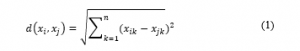
where
d(x_i,x_j ) : Distance between two objects of i and j
x_ik : The value of i object in the k group
x_jk : The value of j object in the k group
Determine the average value of each cluster as follows:

where
T_kj : The average value of the k cluster on the j variable
n : Amount of data
Determine the new centroid closest distance using euclidean distance using (1)
If it doesn’t get the right result, then return to the calculation in step b
The optimum grouping validation uses R-Square and Pseudo F-statistic values. The optimum number of groups can be shown by the highest R-Square and Pseudo F-statistics values [19]. Pseudo F-Statistics values can be calculated by:

The R-Square calculation involves several diversity data calculations, they are total diversity, diversity within groups, and diversity between groups [10]. The value of diversity can be calculated by:

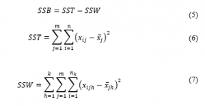
where
SST : Sum of Square Total
SSW: Sum of Square Within Group
SSB : Sum of Square Between Group
m : The number of numerical variables in the observation
k : The number of groups
n : Total number of objects under observation
n_k : Number of members in the k group
x_ij : The value of i object in the j variable
x ̅_j : Average of all j variable
x_ijh : The value of i object in the j variable, and h group
x ̅_jh : Average of all j variable, and h group
K-Modes
K-Modes is the development of the K-Means method specifically used to handle categorical data type cases [20], [18]. This method has an efficient algorithm based on frequency to find modes [21], [18].
Several modifications to the K-Modes method are accommodated from the K-Means method, as follows:
The distance of two data points between X and Y is the number of features found in X and Y. Measuring the similarity between objects X and Y is given by:

Change the means value (average) to mode value (modes)
In searching for mode values, data frequency is used. The centroid point is obtained from each feature’s mode.
The validation method to find out the most optimum grouping in categorical data uses the calculation of the value of r is given by:

where
n : The number of observations
q_h : The highest number of objects (dominance) in the h-group with (h = 1,2,…,k).

Ensemble ROCK
The ensemble ROCK method uses the concept of a link that is used to measure the similarity and closeness that occurs at a pair of data points [22], [23] and [4]. Here are the steps of clustering data by using ensemble ROCK method:
Calculate sim(X_i 〖,X〗_j ) as a measurement of similarity as folllows:

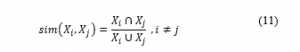
where
X_i : The i group observation group
X_j : The j group observation group
Determine Neighbors by calculating the link value as follows:

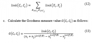
where link(C_i,C_j ) are the number of links of all possible pairs of objects contained in C_i and C_j, and f(θ) is the threshold function obtained, with f(θ)=(1-θ)/(1+θ) where θ (0<θ<1) is a random threshold value determined by the researcher.
Compare the results of clustering from each threshold (θ) researchers have determined.
The validity of ensemble ROCK method can be derived from the ratio of S_w (sum within) and S_b (sum between), (S_w/S_b ). The better grouping performance of the cluster obtained by the smallest ratio of (S_w/S_b ) [18][24]. The value of S_w and S_b is:

SSW and SSB for categorical data can be formulated by:

where
n_ih : The number of observations in the i category, and h group, with h=1,2,3,…,k
n_(.h)=∑_(i=1)^n▒n_ih : The number of observations in the h group
n_(i.)=∑_(h=1)^k▒n_ih : The number of observations in the i category

Research Method

Research data

The research data were obtained from the Central Statistics Agency (BPS) of East Java with the website address https://jatim.bps.go.id/. The data consists of survey data in 2014 and 2018. Data in 2014 as a comparison with the determination of disadvantaged regions in 2015 by the Ministry of Villages, Development of Disadvantaged Regions, and Transmigration. While the 2018 data will be used as predictions to provide an overview regarding the determination of disadvantaged regions next 2020.
This study consists of two types of variables used, namely alternative variables and criterion variables. The alternative variables in this study concern all District/City in East Java Province consisting of 29 District and 9 City according to the details in Table 1.
Table 1: Alternative Research Variables

Code	District/City	Code	District/City
01	Pacitan	20	Magetan
02	Ponorogo	21	Ngawi
03	Trenggalek	22	Bojonegoro
04	Tulungagung	23	Tuban
05	Blitar	24	Lamongan
06	Kediri	25	Gresik
07	Malang	26	Bangkalan
08	Lumajang	27	Sampang
09	Jember	28	Pamekasan
10	Banyuwangi	29	Sumenep
11	Bondowoso	30	Kediri City
12	Situbondo	31	Blitar City
13	Probolinggo	32	Malang City
14	Pasuruan	33	Probolinggo City
15	Sidoarjo	34	Pasuruan City
16	Mojokerto	35	Mojokerto City
17	Jombang	36	Madiun City
18	Nganjuk	37	Surabaya City
19	Madiun	38	Batu City

The criterion variable in this study consists of 6 criteria whose 33 indicators. These variables consist of numeric and categorical data. For criterion variables that are of numerical data type, the determination of disadvantaged regions has 27 indicator variables shown in Table 2.
Table 2: Variable Criteria for Numerical Data

Criteria	Indicator	Source
Regional economy	Percentage of poor population ( )	The Potential of East Java Village
	Population production per capita )
Regional characteristics	Percentage of villages affected by the earthquake	The Potential of East Java Village
	Percentage of villages affected by landslides (
	Percentage of villages affected by floods (
	Percentage of villages affected by other disasters (
	Percentage of protected forest area (
	Percentage of villages conserving critical land (
	Percentage of villages in conflict (
Human Resources	Life expectancy ( )	Human Development Index
	Average school length ( )
	Literacy numbers ( )
Accessibility	Distance from District capital to provincial capital ( )	East Java in Figures
	Number of villages with easy access to security services > 5 km ( )
Infrastructure	Number of villages with the widest asphalt road surface ( )	Potential of East Java Village
	The largest number of villages on the road surface is hardened ( )
	Number of villages with the broadest road surface ( )
	Number of villages with the widest road surface ( )
	Number of market villages without permanent buildings ( )
	Number of health infrastructure per 1000 population ( )
	Number of doctors per 1000 population ( )
	Number of high schools per 1000 population ( )
	Percentage of household electricity users ( )
	Percentage of household telephone users ( )
	Percentage of households that use clean water ( )
Regional Finance	Degree of Fiscal Decentralization ( )
Characteristics of certain regions	Percentage of Disadvantaged Villages )	Human Development Index

Next, for the criterion variable whose categorical data, the determination of disadvantaged regions has 6 indicator variables shown in Table 3.
Table 3: Categorical Data Criteria Variables

Criteria	Indicator	Criteria	Indicator
Characteristics of Specific Regions	Borderland (	0:Not Borderland 1:Borderland	East Java in Figures
	Island existence (	0: Own the island 1: Not an island
	Post-tribal conflict regions ( )	0: There are no conflicts 1: there is a conflict
	Food insecure regions ( )	0: Not a food-insecure area 1: Food insecure regions	Center for Data and Information on Development of Specific Regions of Food-Prone Regions
	Landslide ( )	0: Nothing 1: medium 2: medium height	Regional Planning and Development Agency
	Flood ( )	0: Nothing 1: Intermediate 2: Height
	Earthquake ( )	0: Nothing 1: Yes
	Tsunami ( )	0: Nothing 1: Medium 2: Large
	Volcano eruption ( )	0: Nothing 1: Yes

Data analysis

In this study, data analysis using ensemble ROCK method was carried out with the following steps:
Separate categorical data and numeric data
Reduce research variables with factor analysis both numeric and categorical data
Analyze numerical data clusters using the K-Means method
Validate the optimum grouping using Pseudo F-statistics and R^2
Analyze categorical data clusters using the K-Modes method
Validate the optimum grouping using the calculation of the value of r (highest accuracy)
Analyze mixed data clusters (numeric and categorical) results using the ROCK method

Results and Discussion

Determination of Disadvantaged Regions in 2015
The first step of this research is to cluster data from survey results in 2014 that used as a determination of disadvantaged regions in 2015. For the data processing in this section (in 2014), we don’t elaborate, but we provide detailed discussions for data processing in 2018 in the next sub-section.
The following results of regional clusters in East Java (the data processing in 2014) using the ROCK method can be shown in Table 4.
Based on Table 4, it is known that cluster in disadvantaged regions are Trenggalek, Jember, Banyuwangi, Bondowoso, Situbondo, Probolinggo, Bangkalan, Sampang, Pamekasan, Sumenep, and Probolinggo City, this is in line with the determination of disadvantaged regions conducted by the Government. Based on Presidential Regulation No. 131/2015, it is known that District/City in East Java Province included in disadvantaged regions are Bangkalan, Sampang, Bondowoso, and Situbondo.
Table 4: Clusters of disadvantaged, developing, independent and developed regions

Cluster	District/City
Disadvantaged	Trenggalek, Jember, Banyuwangi, Bondowoso, Situbondo, Probolinggo, Bangkalan, Sampang, Pamekasan, Sumenep, Probolinggo City
Developing	Pacitan, Blitar, Kediri, Pasuruan, Ngawi,  Kediri City, Tuban, Blitar City, Mojokerto City, Madiun City
Independent	Lumajang, Mojokerto, Jombang, Bojonegoro, Lamongan, Gresik, Pasuruan City
Developed	Ponorogo, Tulungagung, Malang, Sidoarjo, Nganjuk, Madiun, Magetan,  Malang City, Surabaya City, Batu City

Predicting the Designation of Disadvantaged Regions in 2020
After the determination of disadvantaged regions in 2015, the next determination will carried-out in 2020. Based on data compiled from the 2018 survey, it can be predicted which regions are potentially designated as disadvantaged regions in East Java. To analyze this case, we use the ensemble ROCK method. In this section, we provide detailed discussions for its data processing.
The first step in the ROCK method is factor analysis. There are several assumption tests in factor analysis, including the adequacy of correlation data between variables using the KMO test and the dependency test between variables using the Barlett test. KMO test results (0.524) >0.50 and Bartlett test obtain sig. (0.000) < (α = 0.05).They show that the research data has fulfilled the correlation and is sufficient to be factored. The results of the factor analysis of numerical data were obtained from the results of factoring and the biggest loading factors. The results of factor analysis for numerical data can be shown in Table 5.
Table 5: Results of numerical data factor analysis

Factor	Indicator	Loading Value
1	The average length of school ( )	0.947
2	Number of high schools per 1000 population	0.784
3	Number of villages with the broadest road surface	0.251
4	Percentage of villages affected by the earthquake ( )	0.745
5	Number of villages with easy access to security services ( )	0.745
6	Percentage of villages affected by flooding ( )	0.420
7	Number of villages with the widest road surface ( )	0.322

The results of the factor analysis will be analyzed and clustered using the K-Means method. In this case, cluster analysis will be carried out into 2,3, and 4 clusters. The selection of an optimal number of clusters is obtained from the largest Pseudo F-statistics and R-Square values. Table 6 is the result of calculating the Pseudo F-statistic and R-Square values for each cluster.
Table 6: R-Square and Pseudo F-Statistic values for each clustering

Number of Cluster	R-Square	Pseudo F-statistic
2 Cluster	0.5680428	47.34160
3 Cluster	0.7443780	50.96045
4 Cluster	0.8258974	53.76237

Based on Table 6 it is known that the optimal number of clusters is 4 cluster. The results of clustering numerical data in the district/city of East Java can be shown in Table 7.
Table 7: Results of cluster using K-Means

District /City	Cluster Result	District /City	Cluster Result
Pacitan	4	Magetan	2
Ponorogo	2	Ngawi	2
Trenggalek	2	Bojonegoro	3
Tulungagung	2	Tuban	3
Blitar	2	Lamongan	1
Kediri	3	Gresik	1
Malang	3	Bangkalan	1
Lumajang	3	Sampang	3
Jember	3	Pamekasan	3
Banyuwangi	4	Sumenep	2
Bondowoso	2	Kediri City	3
Situbondo	2	Blitar City	2
Probolinggo	3	Malang City	3
Pasuruan	1	Probolinggo City	3
Sidoarjo	1	Pasuruan City	1
Mojokerto	1	Mojokerto City	1
Jombang	3	Madiun City	2
Nganjuk	3	Surabaya City	1
Madiun	2	Batu City	3

Then, factor analysis will be carried out for categorical data. The results of the KMO test and the Barlett test for categorical data indicate that the KMO test result (0.683) > 0.50 and Bartlett’s test obtain sig. (0.000) < (α = 0.05). They show that the research data has fulfilled the correlation and is sufficient to be factored. The results of factor analysis for categorical data can be shown in Table 8.
Table 8: Results of categorical data factor analysis

Factor	Indicator	Loading Value
1	Landslide-prone regions	0.818
2	Post-conflict regions	0.874
3	Borderland	0.867

Next, the results of the factor analysis will be analyzed and clustered using the K-Modes method. In this case, cluster analysis will be conducted into 2,3, and 4 clusters. The selection of an optimal number of cluster is obtained from the highest r accuracy value. Table 9 is the result of calculating the accuracy value of r for each cluster.
Table 9: Comparison of the r values for each clustering

Number of Cluster
2 Cluster	0.6666667
3 Cluster	0.7894736
4 Cluster	0.8245614

Based on Table 9, it is known that the optimal number of clusters is 4 clusters. The results of clustering categorical data in the district/city of East Java can be shown in Table 10.
Table 10: Results of cluster using K-Modes

District /City	Cluster Result	District /City	Cluster Result
Pacitan	1	Magetan	1
Ponorogo	1	Ngawi	1
Trenggalek	1	Bojonegoro	3
Tulungagung	2	Tuban	3
Blitar	2	Lamongan	3
Kediri	2	Gresik	3
Malang	2	Bangkalan	1
Lumajang	1	Sampang	3
Jember	2	Pamekasan	3
Banyuwangi	2	Sumenep	3
Bondowoso	2	Kediri City	4
Situbondo	2	Blitar City	4
Probolinggo	1	Malang City	4
Pasuruan	1	Probolinggo City	1
Sidoarjo	2	Pasuruan City	1
Mojokerto	2	Mojokerto City	4
Jombang	2	Madiun City	4
Nganjuk	2	Surabaya City	1
Madiun	2	Batu City	4

After obtaining cluster of categorical and numerical data, the next step is to analyze a mixed data cluster using Ensemble ROCK. In this study, the mixed data will be clustered into 3 and 4 clusters. The threshold values (θ) that will be tested are 10 threshold (θ), they are 0.1; 0.2; 0.3; 0.01; 0.02; 0.03; 0.04; and 0.05. Among the 10 thresholds used, a threshold value which produce the optimum cluster will be chosen by finding the smallest Sw and Sb ratio. The ratio of Sw and Sb from each threshold for grouping 3 and 4 clusters are as follows:
Table 11: Sw and Sb ratio values for each threshold for grouping 3 and 4 clusters

Threshold	3 Clusters	4 Clusters
0.1	0.7237014	0.855867
0.15	0.5414150	0.9331397
0.2	0.4737199	0.5209103
0.25	1.3563698	0.8428222
0.3	0.4157780	0.4938904
0.01	0.5260732	0.8196005

Based on Table 11, it is known that the smallest value of Sw and Sb ratio is owned by the 0.02 threshold with 4 clusters. The results of the mixed data cluster analysis in 4 clusters whose threshold value of 0.02 can be shown in Table 12.
Table 12: Results of the ROCK method cluster (θ=0.02)

Cluster	Cluster Member (District/City)
Cluster 1	Pacitan, Tulungagung, Blitar, Jember, Mojokerto, Jombang, Magetan, Blitar City, Madiun City, Probolinggo City.
Cluster 2	Kediri, Banyuwangi, Nganjuk, Madiun, Bojonegoro, Gresik, Kediri City, Pasuruan City, Mojokerto City.
Cluster 3	Trenggalek, Bondowoso, Situbondo, Probolinggo, Tuban, Bangkalan, Pamekasan, Sumenep, Sampang.
Cluster 4	Ponorogo, Malang, Lumajang, Pasuruan, Sidoarjo, Ngawi, Lamongan, Malang City, Surabaya City, Batu City.

Based on the Regulation of the Minister of Villages, Development of Disadvantaged Regions and Transmigration Number 3 of 2016 concerning Technical Guidelines for Determining Indicators in the Determination of Disadvantaged Regions Article 17 states that in Determining the Direction of Backwardness, it is measured based on positive and negative Composite Index whose values are between +1 and -1 on the criteria. A positive composite index means the higher index of a criterion, the worse condition of a region. Some examples of indicators included in the positive composite index are indicators of the percentage of poor people, the percentage of flooded villages, percentage of villages with critical land. The higher percentage value of those indicators, the worse situation of the region. Conversely, a negative composite index means the lower index of a criterion, the better condition of a region. One example of indicators included in the negative composite index is the average length of the school indicator, the lower value of that indicator, the better condition of the region.
Figure 1 is the percentage group of negative composite levels of each cluster results with the direction of each indicator lags.

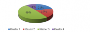
Figure 1: Percentage of Behind Each Cluster

Based on Figure 1, the percentage of negative composite level with the highest backwardness is cluster 3, then followed by cluster 1, cluster 4, and cluster 2. Each cluster result will be grouped successively into disadvantaged, independent, and developed regions. Table 13 is a cluster of disadvantaged, developing, independent, and developed regions.
Table 13: Clusters of Disadvantaged, developing, independent and developed regions

Cluster	Cluster Member (District/City)
Disadvantaged	Trenggalek, Bondowoso, Situbondo, Probolinggo, Tuban, Bangkalan, Pamekasan, Sumenep, Sampang.
Developing	Pacitan, Tulungagung, Blitar, Jember, Mojokerto, Jombang, Magetan, Blitar City, Kota Madiun, Probolinggo City.
Independent	Kediri, Banyuwangi, Nganjuk, Madiun, Bojonegoro, Gresik, Kediri City, Pasuruan City, Mojokerto City.
Developed	Ponorogo, Malang, Lumajang, Pasuruan, Sidoarjo, Ngawi, Lamongan, Malang City, Surabaya City, Batu City.

Discussion

Based on Table 13, it is known that regions designated as disadvantaged regions in East Java consist of Trenggalek, Bondowoso, Situbondo, Probolinggo, Tuban, Bangkalan, Pamekasan, Sumenep, Sampang. It is quite reasonable, some facts compiled from the online mass media reinforce the statement.
In the prediction of setting up disadvantaged regions in 2020, it is known that Tuban has entered into disadvantaged regions. This is because of the percentage of poor people at Tuban increased from the previous year. Based on the news in suarabanyuurip.com (accessed 30-May-2019), the poverty level of Tuban is ranked fifth out of all District/City in East Java [25]. In addition, the percentage of clean water user households in Tuban District is very low, similar to Trenggalek and Situbondo District. Here is a graph of 5 districts/cities that are pockets of poverty in East Java.
On the other hand, based on the Presidential Regulation of the Republic of Indonesia Number 63 the Year 2020 concerning Determination of Disadvantaged Regions in 2020-2024, it was found that East Java has been separated from the provinces with disadvantaged regions. This is possible because local governments have conducted evaluations and various handling efforts to reduce the region of disadvantaged status. Nonetheless, this research result can provide an overview for district/city governments so that they can immediately anticipate and make policies that are adjusted to the characteristics of each region so that their region does not become disadvantaged again.

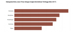
Figure 2: The top 5 poor districts/cities in East Java

Conclusion

The results of clustering using the ROCK ensemble method obtained cluster results for the prediction of disadvantaged regions in 2020 consist of Trenggalek, Bondowoso, Situbondo, Probolinggo, Tuban, Pamekasan, Sumenep, Bangkalan, and Sampang. The best cluster results for evaluating the determination of disadvantaged regions in 2020 consist of 4 clusters with the smallest Sw and Sb ratio of 0.3873984 and the optimum threshold value of 0.04.
The characteristics of each region that are determined as disadvantaged regions, need to be improved to alleviate the area from disadvantages including the level of fiscal decentralization, the percentage of poor population, life expectancy, the average length of schooling, number of health infrastructure, percentage of household electricity users, the percentage of telephone user households, the low percentage of households using clean water, access to the nearest service facility, and the low percentage of protected forest regions.

1. T. Alqurashi, W. Wang, “Clustering ensemble method,” International Journal of Machine Learning and Cybernetics, 2018, doi:10.1007/s13042-017-0756-7.
2. S. Liu, B. Zhou, D. Huang, L. Shen, “Clustering Mixed Data by Fast Search and Find of Density Peaks,” Mathematical Problems in Engineering, 1, 1–7, 2017, doi:10.1155/2017/5060842.
3. S. Vega-Pons, J. Ruiz-Shulcloper, “A survey of clustering ensemble algorithms,” International Journal of Pattern Recognition and Artificial Intelligence, 25(3), 337–372, 2011, doi:10.1142/S0218001411008683.
4. K.S. Sudipo Guha, Rajeev Rastogi, “A robust clustering algorithm for categorical attributes,” Information Systems, 25(5), 345–366, 2000, doi:10.1016/S0306-4379(00)00022-3.
5. M.F. Balcan, Y. Liang, P. Gupta, “Robust hierarchical clustering,” Journal of Machine Learning Research, 15, 4011–4051, 2014, doi:10.1184/r1/6476297.
6. M.V.J. Reddy, B. Kavitha, “Clustering the Mixed Numerical and Categorical Datasets Using Similarity Weight and Filter Method,” International Journal of Database Theory and Application, 5(1), 121–133, 2012.
7. J. Oyelade, I. Isewon, F. Oladipupo, O. Aromolaran, E. Uwoghiren, F. Ameh, M. Achas, E. Adebiyi, “Clustering Algorithms: Their Application to Gene Expression Data,” Libertas Academica Freedom To Research, 10, 237–253, 2016, doi:10.4137/BBI.S38316.TYPE.
8. S. Sharma, Applied multivariate tecnhiques, John Wiley & Sons Inc, New York, 1996.
9. D.H. Setiadi, Pemetaan Kabupaten/Kota di Jawa Timur Berdasarkan Indikator Daerah Tertinggal Dengan Metode Data Campuran Ensamble ROCK dan SWFM, Institut Teknologi Sepuluh Nopember, 2018.
10. Alvionita, Sutikno, Suharsono, “Ensemble ROCK Methods and Ensemble SWFM Methods for Clustering of Cross Citrus Accessions Based on Mixed Numerical and Categorical Dataset,” in IOP Conf. Series: Earth and Environmental Science, 1–10, 2017, doi:10.1088/1755-1315/5.
11. A. Djuraidah, “Evaluasi Status Ketertinggalan Daerah Dengan Analisis Diskriminan,” Seminar Nasional Matematika Dan Pendidikan Matematika Jurusan Pendidikan Matematika FMIPA UNY, 1–16, 2009.
12. S. Wiratama, H.C. Diartho, F.W. Prianto, “Analisis Pembangunan Wilayah Tertinggal di Provinsi Jawa Timur,” E-Journal Ekonomi Bisnis Dan Akuntansi, 5(1), 16–20, 2018, doi:10.19184/ejeba.v5i1.7726.
13. I. Simarmata, A.J.A. Arma, Arnita, “Aplikasi Analisis Faktor dengan Metode Principal Component Analysis dan Maximum Likelihood dalam Faktor-faktor yang Memengaruhi Pemberian Makanan Tambahan Pada Bayi Usia 0-6 Bulan di Desa Pematang Panjang Kecamatan Air Putih Kabupaten Batubara Tahun 2013,” Jurnal Kebijakan, Promosi Kesehatan Dan Biostatistika, 5, 1–10, 2013.
14. H. Suriani, I. Norlita, W.J. Wan Yonsharlinawati, G. Khadizah, B. Kamsia, G. Darmesah, A.S. Asmar Shahira, “Using Factor Analysis on Survey Study of Factors Affecting Students ’ Learning Styles,” International Journal of Applied Mathematics and Informatics, 6(1), 33–40, 2012.
15. H. Schneeweiss, H. Mathes, “Factor Analysis and Principal Components,” Journal of Multivariate Analysis, 55, 105–124, 1995.
16.  A. Field, Factor Analysis Using SPSS, 1–14, 2005.
17. R.A. Johnson, D.W. Wichern, Applied Multivariate Statistical Analysis Sixth Edition, Six, Person Prentice Hall, New Jearsey, 2007.
18. C. Oktarina, K.A. Notodiputro, I. Indahwati, “Comparison of K-Means Clustering Method and K-Medoids on Twitter Data,” Indonesian Journal of Statistics and Its Applications, 4(1), 189–202, 2020, doi:10.29244/ijsa.v4i1.599.
19. A.R. Orpin, V.E. Kostylev, “Towards a statistically valid method of textural sea floor characterization of benthic habitats,” Marine Geology, 225(1–4), 209–222, 2006, doi:10.1016/j.margeo.2005.09.002.
20. Z. Huang, “Extensions to the k-Means Algorithm for Clustering Large Data Sets with Categorical Values Extensions to the k-Means Algorithm for Clustering Large Data Sets with Categorical Values,” Data Mining and Knowledge Discovery, 2(3), 283–304, 1998, doi:10.1023/A:1009769707641.
21. P.S. Bishnu, V. Bhattacherjee, “A Modified K -Modes Clustering Algorithm,” in International Conference on Intelligent Information Hiding and Multimedia Signal Processing, 60–66, 2013, doi:10.1109/IIH-MSP.2014.118.
22. M. Dutta, A.K. Mahanta, A.K. Pujari, “QROCK: A quick version of the ROCK algorithm for clustering of categorical data,” Pattern Recognition Letters, 26(15), 2364–2373, 2005, doi:10.1016/j.patrec.2005.04.008.
23. S. Guha, R. Rastogi, K. Shim, “Rock: a robust clustering algorithm for categorical attributes,” Information Systems, 25(5), 345–366, 2000, doi:10.1016/S0306-4379(00)00022-3.
24. M.J. Bunkers, J. James R. Miller, A.T. DeGaetano, “Definition of Climate Regions in the Northern Plains Using an Objective Cluster Modification Technique,” Journal of Climate, 9(1), 130–146, 1996, doi:10.1175/1520-0442(1996)009<0130:DOCRIT>2.0.CO;2.
25. N.S. Wisnujati, Laporan Pelaksanaan Penanggulangan Kemiskinan Daerah Kabupaten Tuban Tahun 2016, Universitas Wijaya Kusuma Surabaya, Surabaya, 2019

(Click Here)

(Click Here)