1. Introduction

This paper describes a modification of a text encoding algorithm, presented at ICASC 2019. Since the conference proceedings paper [1] was written, there have been further developments and those will be presented here, but first a bit of backstory.

One of the most prolific research teams, who currently experiment with sparse distributed representations (SDR), are Jeff Hawkins, Subutai Ahmad [2] and the people working with them at the private company Numenta. The principle author of this paper found out about the concept of SDR from their work and drew inspiration from their research.

An important thing to note, is that the long term goal of the researchers at Numenta is to distance their developments from conventional machine learning and artificial neural networks. We do not share this goal, in fact we are merely trying to make solutions based on sparse information representation, which are complementary to classic machine learning.

Here we present a type of encoder for text data, which is not described in the research paper on sparse encoders, published by a member of Numenta [3]. Our solution is also different from the Cortical.io SDR text encoder, which is mentioned in point 6 of the Numenta paper (Webber, “Semantic Folding”). We follow the principles described in the conclusions of the Numenta research paper, but the algorithms and implementation are entirely our own. The data structures we use are not binary arrays, we use key-value data structures to implement the representations. Compared to other SDR text encoders, another notable difference in our approach is that we consider characters to be the basic building units of text, not abstract constructs such as words.

This paper focuses on a key enhancement made to our algorithm, presented at ICASC, and the potential benefits it offers. It also covers the development of a benchmark text classification problem, for evaluating the utility of our text encoding algorithms, by comparing them to conventional text vectorizers.

To avoid confusion, our initial algorithm will be referred to as CP (Current-Prior). The modified one, which is the focus of this paper, will be referred to as CPPP (Current-Position-Prior-Position). Their names hint at the way in which they transform strings into sparse distributed representations.

2. Comparing CP and CPPP sparse representations

In brief, CP encoding goes through strings character by character and uses only their sequencing to create a sparse representation of the strings in a two-dimensional encoding space. For a more detailed description of each step, please refer to the ICASC paper. The encoding space is an abstract concept and one of its key features is that the coordinate system uses non-numeric characters, to define the location of points within the space. As the CP encoder moves from character to character, it projects the last character it has read onto the horizontal axis, but it also uses the vertical axis to track prior characters. This is why the algorithm is called current-prior. The result is a specific pattern of points in the encoding space, which is highly dependent on the symbol arrangement of the strings being processed.

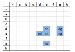
Figure 1: edge (CP encoded)

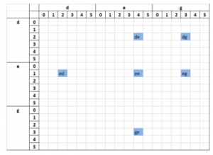
Figure 2: edge (CPPP encoded)

      The encoding patterns can be illustrated in various ways, with one of the more human-readable ones being tabular representation, as seen on Figure 1. If the representations are being processed by a computer program, however, there are more suitable data structures, which could be used. For example, the CP encoded word shown in Figure 1 can be stored as a set of character pairs:
{‘ e’, ‘ d’, ‘ g’, ‘  ‘, ‘ed’, ‘eg’, ‘ee’, ‘e ‘, ‘dg’, ‘de’, ‘d ‘, ‘ge’, ‘g ‘}.

      CPPP encoding works in a similar way, but in addition to character sequences it also factors in the position of the characters. In other words, the sparse encoding space has two additional sub-axes, which track the positions of the last read symbol and the position of prior symbols. Even though this defines a four-dimensional encoding space, it can still be represented in tabular form (Figure 2). This is the key modification to the CP algorithm and it is noted in the name (Current-Position-Prior-Position).

      In theory, the readability of these tables does not diminish, because the encoded strings are sparse patterns by definition. The repetition of the sub-axes below the main axes doesn’t make the tabular representation harder to interpret. It still looks like a grid with seemingly random non-empty elements scattered throughout. There is actually nothing random about the distribution of the non-empty elements, however. It is strictly based on the encoded string.

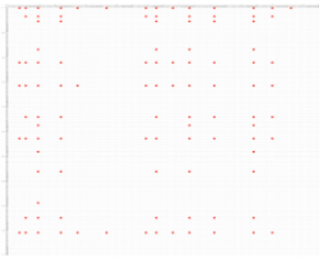
Figure 3: The phrase “when it rains”, encoded with CPPP

      Difficulties could arise in practice, because of the size of the string being encoded. The sparse representation is still logical and consistent, it is just not possible for a human to comprehend what it means at a glance (Figure 3).

      However, these algorithms are meant to be utilized by computers, not people. Machines are far better at processing large amounts of information. The ability to represent the encodings in a human-readable format is useful mainly to the developers, as a debugging tool and a way to illustrate the working principles of these algorithms.

3. Pseudocode implementation

3.1. Input-output

strIn – The string which has to be transformed into a sparse representation. It can be of arbitrary length.

SR – The output from the encoding procedure, i.e. the sparse representation of the input. It is just a key-value data structure. We used python dictionaries, but any other dictionary-like data structures from other languages can be used to implement the algorithms.

winSize – A control parameter, which sets the maximum allowed distance between characters, when forming character pairs.

For example, when encoding an entire book, it would make little sense to form pairs from characters at the start of the book and characters at the very end of the book. That would just create more character pairs (points in the encoding space) than is necessary and significantly increase the size of the sparse representation.

We used winSize = 20, i.e. we told the program not to form points from characters, which were separated by more than 20 characters.

3.2. CP encoding algorithm

Algorithm 1: Current-Prior
Result: SR
Receive strIn; Initialize dictionary object SR; prior_pos = 0;
while prior_pos < length of strIn do
	current_pos = prior_pos + 1;
	while current_pos < length of strIn do
		chrPair = Concat(strIn[prior_pos], strIn[current_pos]);
		SR[chrPair] = 1;
		current_pos += 1;
	end
	prior_pos += 1;
end

3.3. CPPP encoding algorithm

The keys in the CPPP sparse representation key-value data structure are derived in the same way as the ones produced by CP encoding. However, the values are not just a single number. The values are lists of numbers, specifically the positions of the characters, which produced the keys of the dictionary.

Algorithm 2: Current-Position-Prior-Position
Result: SR
Receive strIn; Initialize dictionary object SR; prior_pos = 0;
while prior_pos < length of strIn do
	current_pos = prior_pos + 1;
	while current_pos < length of strIn do
		chrPair = Concat(strIn[prior_pos], strIn[current_pos])
		if chrPair not in keys of SR then
			SR[chrPair] = list(empty list, empty list);
			append current_pos to list SR[chrPair][0];
			append prior_pos to list SR[chrPair][1];
		end
		current_pos += 1;
	end
	prior_pos += 1;
end

4. Advantages and disadvantages of CPPP

When processing repeating syllables and characters, the CP algorithm projects them in the same points of the sparse encoding space. In contrast, CPPP ensures that each repeating symbol will be projected to a different point in the encoding space. A direct consequence of this is that CPPP encoding can handle strings with arbitrary lengths, whereas CP cannot.

It is possible to saturate the two-dimensional encoding space used by the CP algorithm, if a sufficiently long string is processed. CPPP can transform large strings, without decreasing the sparsity of their representations in the four-dimensional encoding space. The significant advantages of this are:

• Reversible encoding. It is possible to turn the sparse representations back into strings, without information loss.
• No need for tokenization. Text documents (data) can be processed as a single, long, uninterrupted sequence of characters. There is no need for splitting them by delimiters, such as whitespace, commas and such.
• Increased capacity. Due to the introduction of the two additional dimensions, for tracking character positions, it is possible to compare not only tokens (words), but entire sentences, phrases, paragraphs and documents.
• Precise string comparison. CPPP allows not only the quantification of similarity between strings, but it also makes it possible to determine which specific parts of the strings correspond to each other and which ones differ.

Despite the advantages, the modified algorithm has a notable drawback: the simple methodology for comparison of CP sparse representations is not applicable to CPPP encoded text.

To illustrate the reason, several words encoded by the two algorithms will be examined. The chosen words are tree, trim and tree-trimmer, because these words are short, some of them have double characters and the third one is a compound word, which includes the other two.

CP encoding (Figures 4 to 6) does not represent the following things properly:

• The double е in tree and the double m в trimmer. In both cases, the corresponding points for these characters in the encoding space overlap. For the word tree, the points are re and te. For trimmer, the points are im, rm and tm.
• The repetition of tr in tree-trimmer (Figure 6). Again, the representations of the two different instances of this character sequence overlap completely in the two-dimensional encoding space. This means that the initial string cannot be recovered, by using only its sparse representation.

Figure 4: tree (CP encoded)

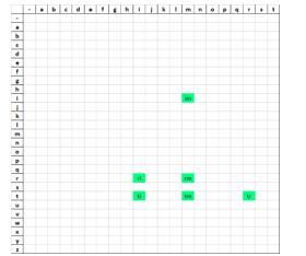
Figure 5: trim (CP encoded)

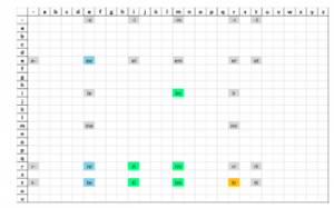
Figure 6: tree-trimmer (CP encoded)

On the other hand, CPPP encoding creates mirror points, when representing repeating character sequences. An example of this can be seen on Figure 7, arrows have been drawn to bring attention to the points in question. They indicate, that the letter е is present more than once in the word tree. The fact that sectors re and te have more than one non-empty value is informative, although the algorithmic processing of this information is not as trivial, as the procedure used to compare sparse patterns in CP encoded strings.

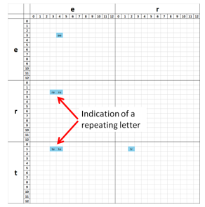
Figure 7: tree (CPPP encoded)

Figure 8: trim (CPPP encoded)

A second complication inherent in CPPP encoding is illustrated on Figures 8 and 9. The points which represent the word trim have shifted their positions in the sparse space. This is to be expected, in the third string there is another word before trim, which causes a translation of the sparse pattern to the right. This is logical and informative, but again, the algorithmic analysis and quantification of such relations is more complex than the one employed for CP sparse representations of text.

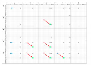
Figure 9: tree-trimmer (CPPP encoded)

      These two characteristics of the modified encoding space (mirror points and non-stationary sparse patterns) are the things that give it the aforementioned advantages. However, there is no analogue for them in the two-dimensional encoding space, which means the comparison method developed for CP sparse representations is not applicable to four-dimensional encodings of strings. To utilize the full potential of CPPP encoding, other comparison techniques have to be used.

5. Methods for comparing CPPP sparse representations

In theory, it is possible to feed the encoded strings into artificial neural networks and have them learn to recognize the same types of patterns, which people can notice in small sparse representations. However, in recent years the European Union has begun to implement legal frameworks and guidelines for the use of artificial intelligence, which emphasize the need for algorithmic transparency (see the publications from 2019 by the EPRS, such as “A governance framework for algorithmic accountability and transparency”).

It is the opinion of the authors, that the more society delegates decision making to machines, the more the legal regulations and requirements for decision transparency will increase. Conventional ANN are black-box approaches to modelling data and as such, the authors try to avoid relying on them, in favor of more algorithmically transparent models. In addition, it is possible to logically and methodically explain why each element of a CPPP sparse representation exists in the encoding space.

In order to make use of the encoded data, however, specialized procedures have to be developed, for quantifying similarities between encoded strings, as well as processing larger units of written information, such as documents, chapters in books etc. To be more specific, text classifiers based on the bag-of-words approach require accurate word/token counts, in order to build quality TF-IDF representations of textual data. Other machine learning approaches, such as n-gram modelling, require tracking of token sequences as well, in order to take into account the context in which individual words are used in the text.

The methods for distinguishing and locating words in CPPP encoded corpora are currently under development, their implementations could change. However, brief examples will be given, to showcase possible ways of carrying out basic operations with CPPP encoded text.

5.1. Basics of locating words in CPPP text representations

The text is CPPP encoded as a single, uninterrupted string. In addition, the computer has access to a machine-readable dictionary, which consists of separately encoded words. Note the different way of encoding the data and the dictionary. Unlike common practice, tokenization of the dataset is avoided, the text is kept intact and it is CPPP encoded as a whole. This is because it is not known which parts of the text correspond to which words, before some kind of analysis is done. This approach avoids the presupposition, that the text being processed is well formatted and can easily be parsed with a few simple delimiting characters.

The dictionary, however, is a collection of distinct words, by definition, so it is divided into separately encoded strings. It is also possible to curate the dictionary manually and ensure the entries are properly separated, something which usually isn’t practicable with the dataset.

5.2. Word search based on maximizing pattern overlaps

For each element (word, token, phrase) in the machine-readable dictionary, the following steps are carried out: finding all potential locations of the search term within the text and filtering the possible results, to leave only the most consistent matches.

5.2.1. Initialization of a character weight vector W.

The purpose of W is to indicate which parts of the text correspond to the dictionary entry, which is under consideration during the entry enumeration. It is initialized as an all-zero vector, with a length equal to the number of characters in the text being analyzed. The first element of W indicates how many times the first character takes part in forming character pairs, which are common to both data and dictionary sparse representations. The second element of W indicates the same for the second character of the text. The third element covers the third character etc.

5.2.2. SPOQ procedure – pseudocode implementation.

The current implementation of the Sparse Pattern Overlap Quantification Procedure, or SPOQ for short, is described here (algorithm 3). It is used to find similar patterns in the encoded data. SR_1 is the sparse representation of the data, SR_2 is a sparse representation of a specific dictionary entry.

Algorithm 3: SPOQ
Result: WSPOQ Initialize W vector with all zero elements;
commonKeys = Intersection(keys of SR_1, keys of SR_2);
for each com in commonKeys do
	crnt_pos1 = SR_1[com][0];   prev_pos1 = SR_1[com][1];
	crnt_pos2 = SR_2[com][0];   prev_pos2 = SR_2[com][1];
	delta1 = crnt_pos1 – prev_pos1;
	delta2 = crnt_pos2 – prev_pos2;
	for each b in delta2 do
		proximity = abs(delta1 – b);
		W[ crnt_pos1[ index of min(proximity) ] ] += 1;
		W[ prev_pos1[ index of min(proximity) ] ] += 1;
	end
end

5.2.3. SPOQ example.

If we look at the sparse representations shown on Figures 8 and 9, their encoding spaces can be divided into sectors (denoted S_T and S_D respectively), by using the primary axes (the ones that track character sequencing). These sectors correspond to the common keys between the two sparse representation data structures. For those sectors, which are not empty and present in both representations, the distances ∆p_T and ∆p_D are calculated. They indicate how far apart specific pairs of characters are in both representations. For details, see Table 1.

The example shown in Table 1 assumes that the word trim is a word from the machine-readable dictionary and tree-trimmer is the text. The elements of the weight vector are incremented, based on the closest matches between ∆p_T and ∆p_D in each sector. This is why indices 6,7,8 and 9 of W will have the highest non-zero values. They correspond neatly to the location of the word trim, within the string tree-trimmer.

Note that this is a relatively simple procedure and it can produce false positives. The fact that index 1 and 2 also get incremented once is an example of the limitations of SPOQ. In addition, there is no guarantee that all relevant characters will be matched properly.

Table 1: Principle of operation of the SPOQ procedure

ST		SD		Incrementations of W
ri	3 – 2 = 1	ri	8 – 2 = 6
		ri	8 – 7 = 1	W8 += 1  and  W7 += 1
ti	3 – 1 = 2	ti	8 – 1 = 7
		ti	8 – 6 = 2	W8 += 1  and  W6 += 1
im	4 – 3 = 1	im	9 – 8 = 1	W9 += 1  and  W8 += 1
		im	10 – 8 = 2
rm	4 – 2 = 2	rm	9 – 2 = 7
		rm	9 – 7 = 2	W9 += 1  and  W7 += 1
		rm	10 – 2 = 8
		rm	10 – 7 = 3
tm	4 – 1 = 3	tm	9 – 1 = 8
		tm	9 – 6 = 3	W9 += 1  and  W6 += 1
		tm	10 – 1 = 9
		tm	10 – 6 = 4
tr	2 – 1 = 1	tr	2 – 1 = 1	W2 += 1  and  W1 += 1
		tr	7 – 1 = 6
		tr	7 – 6 = 1	W7 += 1  and  W6 += 1
		tr	12 – 1 = 11
		tr	12 – 6 =  6

5.2.4. Filtration of weak matches

The SPOQ search procedure described in points 5.2.2 and 5.2.3 is supposed to generate rough estimations of word positions, within a given text. False positives and overlaps between the weight vectors of multiple dictionary entries are to be expected. Currently, it is assumed that these can be handled with adequate filtration techniques.

Regarding how the filtration of each weight vector is done, the code for the SPOQ procedure was described in point 5.2.2, it is the one which produces the initial W vectors, denoted as W_SPOQ. Point 5.2.5 covers the code for the filtration steps, which further modify W_SPOQ.

5.2.5. Pseudocode of the filtration procedures.

Algorithm 4: Frequency filtration
Result: WF
W = WSPOQ;  #input W[W == 1] = 0; N = length of W – 2; cp = 1;
while cp <= N do
	if W[cp-1] == 0 and W[cp] != 0 and W[cp+1] == 0 do
		W[cp] = 0;
	end
	cp += 1;
end

Algorithm 5: Match length filtration
Result: WL
W = WF;  #input likely_loc = integer sequence from 0 to length of W; Keep only the elements of W where W > 0; W_filtered = zero vector of length W; i = 0; j = 1;
while j < length of W do
	if likely_loc[j] – likely_loc[j-1] != 1 then
		substring_size = likely_loc[j-1] – likely_loc[i];
		if substring_size > 2 then
			# This substring is a good match, it is long enough
			W_filtered[ likely_loc[i]: likely_loc[j-1] ] = 1;
		else
			# Bad match, substring is too short
		end
		i = j
	end
	j += 1
end

5.3. Visualization of SPOQ and W filtration.

To visualize the values of the character weight vector, as it is altered by the filtration steps, we utilize custom plots. In addition to W, they display the actual text under evaluation, so that we can quickly determine if the values of W are as they should be.

The layout of the custom plots is described in Figure 10. For specific example with data, refer to Figures 11 to 14 and point 5.3.1, which describes what those figures illustrate.

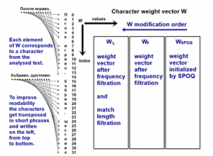
Figure 10: Description of custom plot layout

5.3.1. Example of SPOQ and W filtration used on text

To illustrate the filtration process, the Bulgarian poem “Поточе” (Stream), written by Elin Pelin, will be used as an example dataset. When searching for the word песни (songs), the SPOQ procedure is used to obtain an initial weight vector W_SPOQ, shown on Figure 11.

Figure 11: search for песни

The largest peak in W_SPOQ is roughly equal in size to the length of the search word, about five in this case. As expected, the biggest peak is roughly where the word is in the poem, but there are many other smaller peaks scattered around it. This is why additional filtration steps are necessary.

Many of the individual elements in W_SPOQ are equal to 1 or are surrounded by zeros on both sides. Using the frequency filtration procedure, we zero-out all of these and get a clearer indication of where the search-word is, as shown on Figure 11, subplot W_F. Unfortunately, some false positives still remain.

An additional filtration step can be applied, this time targeting the lengths of the matches. Presumably longer sequences of non-zero values indicate better matches. If we zero-out all matches shorter than 2 characters, we obtain the result seen on Figure 11, subplot W_L. This is indeed where the word is in the document.

5.3.2. Necessary refinements to SPOQ and filtration.

There is a caveat to the simple filtrations described here. Their thresholds are static hyper-parameters, meaning they were set by a person at some point and are not necessarily a good fit in all possible word search cases.

For an example of this, refer to Figure 12, which shows the search for the word песен (song). This is the singular form of the word and a more likely entry in a properly curated dictionary. In this case, the match is weaker and a small increase in the threshold of the length filter (from 2 to 4) could zero-out the entire weight vector, thereby suppressing the one relevant match in the dataset.

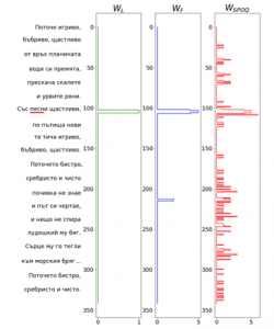
Figure 12: search for песен

The filtration thresholds have to be dynamically adjustable by an automated subroutine. Manual adjustment would not be practicable, considering the number of word searches and comparisons that have to be done in an adequately sized corpus.

A single search in the encoded text could produce multiple results, if the search-word is present in the data more than once, as seen on Figure 13. However, multiple results for a single search could also contain false positives, due to the nature of the algorithm.

Figure 14 shows an example of false positives making it through both filtration steps. The reason for this is that the search-word бистро (pure) is contained nearly unchanged in the word сребристо (silvery). This is why the filtered weight vector has 4 peaks, instead of just 2, which is the correct number of occurrences of the search-word. Finding similar character sequences is the intended behavior of the program, but they aren’t always a correct match.

Work is still ongoing on the development of dynamic filtration, capable of resolving the issues caused by false positives and ambiguities arising from overlaps between the weight vectors of different dictionary entries. Formulating the problem as an optimization procedure is under consideration, the idea being that this way it will be possible to automatically reach a single interpretation of a given corpus. The aim is to produce a data preparation module, based on CPPP encoding. It should be capable of replacing conventional data preparation steps, such as tokenization, stemming, lemmatization, as well as give sufficiently accurate word counts and position estimations.

Figure 13: search for щастливо

Figure 14: search for бистро

6. Text classification benchmark

In order to conduct a more rigorous evaluation, of the performance and quality of CPPP data preparation, a classification problem has been defined, by using a dataset from the LSHTC challenges ^[4]. Specifically, the small wikipedia dataset from LSHTC3 was used, since it was the only challenge in which the raw text was provided.

The dataset has 456886 documents, each one containing only abstracts of wikipedia articles. The documents are labeled, although the labels are not human readable, they are merely integers representing a specific topic covered in each document. There is also a complex label hierarchy, however for the purposes of our benchmark problem, we do not take it into account. We only use a subset of the entire corpus, which contains documents with a single label. In addition, we alter the labels to reduce everything to a binary classification problem. This way we can train a simple model and focus on the data preparation part of the workflow. The aim is to make changes only in the data preparation stage, the text classifier itself will always be the same, with fixed hyper-parameters.

6.1. Subsetting the dataset and forming binary labels

Looking only at the documents with a single label, the top 10 most frequently occurring label codes are listed in Table 2. Next to the codes are descriptions, based on reading and evaluating a dozen of the documents associated with a given label.

Table 2: Top 10 most used labels

Label	Documents	Label Description
167593	5277	Movies
347803	1470	Businessmen and inventors
324660	1433	Historic buildings
283823	1359	Writers and journalists
284433	1310	Journalists
272741	1006	Film actors
395447	999	Screenwriters
114873	945	Plants
352578	846	Novelists
93043	762	Painters

Label 167593 was chosen as the positive class (the one we want to predict with the model). The decision was based solely on the number of documents tagged with 167593. To create the benchmark corpus, all documents with the chosen label were selected, and reassigned to class 1. An additional 4000 randomly chosen documents, from the remaining 451609 in the dataset, were assigned to class 0, regardless of what their labels were originally. This is how the initial classification of the documents was reduced to a binary classification problem.

In addition, a variable was added to the subset, which randomly separates it into two roughly equal in size parts. This is used to perform a training-validation split, for when the text classification model is trained on the subset.

The only preprocessing of the raw text was the removal of punctuation and the substitution of numbers with the placeholder <NUMBER>. Other preprocessing steps, such as named entity recognition, have not been implemented, although they are under consideration.

Note that for statistical purposes, this procedure was repeated 30 times, to produce 30 distinct subsets, each with different documents assigned to the negative class 0 and different training-validation splits. The number 47 was used as a seed for generating 30 random numbers, which in turn were used as seeds when the subsets were created. This ensures repeatability of the process. The pseudocode for creating subsets is included (Algorithm 6).

Algorithm 6: Procedure for subsetting the LSHTC3 dataset
Result: Document subsets
# Parameters for subset generation
ran_stat = 47;				# keep constant, used as seed
num_of_subsets = 30;				# Can be varied
N_neg = 4000;				# Can be varied
train_test_ratio = 0.5;				# Can be varied
Load dataset (Dw)
Separate docs for positive and negative class (Dn and Dp);
# Generate a list of random integers rand_int_list = generate_random_integers(
	max value = 1000000,
	length = num_of_subsets,
	seed = ran_stat
);
for each rand_int in rand_int_list do
	Randomly sample (seed = rand_int) N_neg documents from Dn;
	Append Dn_sample to Dp to get subset Ds;
	Remove punctuation in Ds; Replace numbers with <NUMBER> in Ds;
	Add train-test separation flag to Ds(seed = rand_int);
	Save the subset Ds as “subset_<rand_int>.csv”;
end

6.2. Corrupting the text

In order to test whether CPPP encoding can provide more robust data preparation than conventional techniques, each of the created subsets had its documents subjected to varying degrees of text corruption. Note that this only affects the documents used for model validation, the training documents were untouched. The types of text corruption used are:

• D – character deletions. Example: word becomes wrd.
• I – character insertions. Example: word becomes wyozrds.
• B – character blurring. Repeating one or more character in the string many times. Example: wworrrd.

      These three basic types of corruption can be combined together in 7 meaningful ways (___, __I, _D_, _DI, B__, B_I, BD_, BDI), if we allow for the possibility that one or more of them can be inactive. The inactive ones are indicated by an underscore.

      In addition, it is possible to regulate the number of affected words in a document, as well as the severity of text corruption. Table 3 shows examples of the codes used to denote corruption type and severity and explains how to interpret them.

Table 3: Corruption code examples

Corruption code	Interpretation
___ 000 000 0011528	No corruption, use the subset derived from seed 11528.
__I 001 005 0367540	Insert extra characters, at most 1 per word, for 5% of the words in each document. Use the subset derived from seed 367540.
B_I 009 001 0815602	Blur and insert characters, at most 9 per word, for 1% of the words in each document. Use the subset derived from seed 815602.

      Generating the corrupted subsets is done automatically by the benchmark application, which enables the systematic production of thousands of datasets, with varying degrees of corruption. This procedure has a longer code implementation than the algorithms described so far, which is why it has been split into two parts for ease of readability.

      The inner word corruption procedure (Algorithm 8) is the one, which actually changes the words/tokens. The outer corruption procedure (Algorithm 7) is the one which tokenizes the documents and selects which words/tokens in which documents to corrupt. The outer corruption procedure also cycles through all test documents and generates different corruption possibilities, depending on three parameters:

• CT – corruption type (see the start of 6.2);
• NCA – number of characters to alter per word;
• NWD – number of words to alter per document.

      Note that the user does not simply specify the values of these 3 parameters, the user provides several valid values for each of them. The benchmark application determines all relevant parameter combinations by itself.

Algorithm 7: Outer word corruption procedure
Result: Corrupted document subset
Load subset file; Determine which documents are for training and testing; Extract rand_int from the subset name, it will be used as a seed for the random number generator;
ParamCombinations = VaryParameters(
	valid_values_for_CT,
	valid_values_for_NCA,
	valid_values_for_NWD
);
for each parameter combination in ParamCombinations do
	for each docTxt in documents for testing do
			Tokenize docTxt;
			indeces_of_words = randomly select words to alter;
			for each wrd_ind in indeces_of_words do
					Call the inner word corruption procedure;
			end
	end
end
Algorithm 8: Inner word corruption procedure
Result: A single corrupted word/token
Read parameters from the outer procedure; Read docTxt and wrd_ind (indexes the target word);
Randomly select only one type of text corruption to use;
# Select positions in the word for corrupting randomly max_index = length of doc_txt[wrd_ind] – 1; wrd_seed = rand_int + max_index + Unicode code point of first character + Unicode code point of last character;
if max_index == 0 do
	positions = list with one element (index 0);
Else
	positions = generate_random_integers(
			from 0 to max_index,
			length = chars_to_alter,
			seed = wrd_seed
	);
End
if corruption_type is D do
	if length of positions > 1 do
			Leave only unique values in positions list;
			Sort positions list in descending order;
	End
	for each pos in positions do
			delete character at pos in doc_txt[wrd_ind];
	End
End
if corruption_type is I or B do
	if corruption_type is I do
			if length of positions > 1 do
					Sort positions list in descending order;
			End
			seed = wrd_seed; chars2ins_length = chars_to_alter;
			chars2ins = random Unicode code points (32 to 126);
	End
	if corruption_type is B do
			chars2ins = empty list
			for each pos in positions do
					Append Unicode code point of doc_txt[wrd_ind][pos] to chars2ins;
			End
	End
	i = 0
	while i < length of positions do
			insert chars2ins[i] into positions[i] of doc_txt[wrd_ind];
			i += 1
	End
End

6.3. Predetermining computation requirements

      If processing time or memory is an issue, the total number of corrupted datasets Dc can be calculated beforehand with an equation (1).

where:

• N_S – Number of initial subsets.
• C – The number of meaningful combinations of the basic types of text corruption.
• A_C – The number of character alteration levels.
• A_W – The number of word alteration levels.

      As mentioned earlier, we prepared an example with 30 distinct subsets from the full corpus. If we want to alter 1, 3 and 9 characters per word for 1, 5, 20, 50, 80 and 95 percent of the words in each document, then:

                A_C = |{1, 3, 9}| = 3

                A_W = |{1, 5, 20, 50, 80, 95}| = 6

      Thus, the application would produce 30*(1+7*3*6) = 3810 distinct subsets, all with varying types and severity of text corruption, within the desired ranges.

6.4. Training the text classifiers

The Python module scikit-learn was used, specifically the TfidfVectorizer object for feature extraction and the RandomForestClassifier object for creating the text classification models. A distinct model is trained on each of the subsets. Their hyper-parameters are fixed, so any change in prediction quality is due entirely to the dataset, nothing else. The feature extractor and model were trained only on the training data, the validation data was only used to generate class predictions.

The hyper-parameters of the TfidfVectorizer are as follows:

• stop_words = ‘english’
• analyzer = ‘word’
• vocabulary = None
• binary = True
• max_df = 1.0
• min_df = 1
• use_idf = False
• smooth_idf = False
• sublinear_tf = False

The hyper-parameters of the random forest classifier were the default ones, the only parameter we explicitly specified was random_state. This was set equal to the final number in the corrupted subset names (see Table 3). This number is the seed used to generate the subset. Using it as the seed for the model ensures that the random forest algorithm will produce consistentl results for each subset file, no matter how many times the benchmark is executed.

6.5. Evaluating the benchmark results

As expected, models evaluated with uncorrupted or lightly corrupted datasets perform very well, models tested with moderately corrupted documents perform worse and the ones tested with text with severe corruption perform the worst of all.

The full table of classification results is 3810 rows, too large to be included in this paper. Only a snippet is included (Table 4) to show what the format of the output looks like. The full table is summarized with charts in point 6.6.

Table 4: Excerpt from the classification results table

CT	NCC	PWC	Seed	TP	TN	FP	FN
___	0	0	189191	2525	1891	107	95
BDI	3	1	265329	2543	1844	136	96
BDI	3	5	11528	2422	1800	213	169
BD_	1	20	265329	1303	1865	1376	75
BD_	1	50	11528	2387	1247	248	722
B_I	3	95	265329	269	1886	2410	54
B_I	9	1	11528	2520	1866	115	103
_D_	9	95	11528	2380	1436	255	533
_D_	9	5	889991	2513	1905	141	80
_D_	9	50	616169	1321	1880	1327	90
_DI	9	20	837510	1459	1889	1170	82
__I	1	5	998096	2482	1868	146	127
__I	1	20	11528	2348	1826	287	143

Table header descriptions:

• CT – text corruption type.
• NCC – Number of characters altered per word.
• PWC – Percentage of words affected in each test
• Seed – The random number generator seed, which was used to create the initial subset and to alter the text.
• T_P – true positives.
• T_N – true negatives.
• F_P – false positives.
• F_N – false negatives.

6.6. Visualizing the benchmark results

In order to visualize the classifier results in a more compact manner, two things were done with the full results table. First, all T_P, T_N, F_P and F_N were averaged and grouped by CT, NCC and PWC. This effectively combines the results for all of the 30 distinct seeds/subsets which were used. The aggregated results table is reduced to only 128 rows as a result of this summarization.

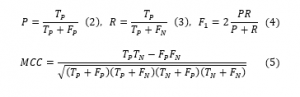
The second step is quantifying the quality of the classification models. Two metrics were calculated, the first one of which is the widely used F₁ score (4), which is just the harmonic mean of the Precision (2) and Recall (3) metrics. The other quality metric is the Matthews correlation coefficient MCC ^[5], which is specifically designed to give more reliable evaluations for binary classification results (5).

The resulting charts are shown on Figures 15 to 28. Note that the Percent of Words Changed per test document (PWC) is on the x-axis, the classification quality metrics are on the y-axis and there is a separate line for each of the 3 levels of word corruption used (1, 3 and 9 character alterations per word).

From the charts it is evident, that there is a consistent downward trend of model quality versus PWC, regardless of the way in which the datasets were corrupted. An interesting thing to note is that MCC is more sensitive than the F₁ score. This, combined with the fact that it gives reliable results, even when the class sizes are imbalanced, makes it the preferred model evaluation metric by the authors.

A detailed comparison between the many text corruption approaches is beyond the scope of this paper. What matters is that the overall trends are the same, regardless of the exact manner in which the test texts were damaged.

The intent here is to describe the benchmark classification problem, which will serve as an evaluation tool for the quality of the custom data preparation tools, based on CPPP encoding. The experimental setup might change (more granulated levels of PWC, more subsets etc.). Once the custom data preparation solution is more mature, it will be evaluated alongside the conventional feature extraction objects from the nltk package in Python.

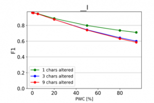
Figure 15: Effect of character insertions on classification quality

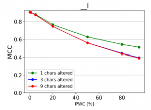
Figure 16: Effect of character insertions (MCC)

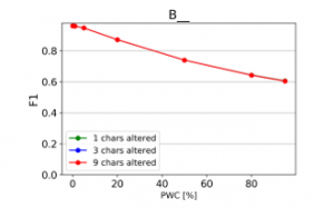
Figure 17: Effect of character repetitions on classification quality

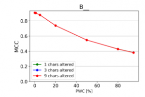
Figure 18: Effect of character repetitions (MCC)

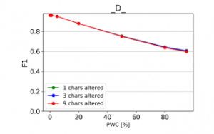
Figure 19: Effect of character deletions on classification quality

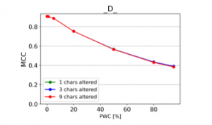
Figure 20: Effect of character deletions (MCC)

Figure 21: Effect of character repetition and insertion on classification quality

Figure 22: Effect of character repetition and insertion (MCC)

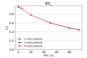
Figure 23: Effect of character repetition and deletion on classification quality

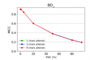
Figure 24: Effect of character repetition and deletion (MCC)

Figure 25: Effect of character deletions and insertions on classification quality

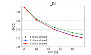
Figure 26: Effect of character deletions and insertions (MCC)

Figure 27: Effect of character repetition, deletion and insertions on quality

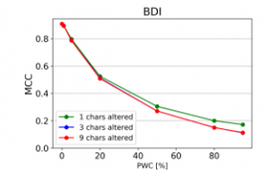
Figure 28: Effect of character repetition, deletion and insertions (MCC)

7. Conclusions

The CPPP text encoding algorithm has notable advantages over the initial CP algorithm. The significant ones are:

• drastically increased capacity of the encoding space;
• corpora don’t have to be tokenized with delimiters;
• the ability to create sparse representations of words, phrases, sentences, paragraphs and even entire documents.

The CPPP algorithm also has advantages over conventional text vectorizers, which rely on tokenization, stemming and other rudimentary techniques of parsing out individual words in a text. The current versions of the string comparison subroutines (SPOQ and its associated filtrations) were presented in the paper. These will be developed further, in order to fully utilize the potential of the sparse representations, produced by the CPPP algorithm.

The benchmark classification problem, described at the end of the paper, will help guide the ongoing development effort. It will also enable comparisons to be made with conventional solutions for data preparation and feature extraction, by using widely known and reliable classification quality evaluation metrics.

Conflict of Interest

The authors declare no conflict of interest.

Acknowledgment

The authors would like to thank Technical University of Sofia – Research and Development Sector, for their financial support.

1. M. Marinov and A. Efremov, “Representing character sequences as sets : a simple and intuitive string encoding algorithm for NLP data cleaning,” in 2019 IEEE International Conference on Advanced Scientific Computing (ICASC), 1-6, 2019, https://doi.org/10.1109/ICASC48083.2019.8946281
2. Subutai Ahmad, Jeff Hawkins, “Properties of Sparse Distributed Representations and their Application to Hierarchical Temporal Memory”, Cornell University, 2015, arXiv:1503.07469
3. Scott Purdy, “Encoding Data for HTM Systems”, Cornell University, 2016, arXiv:1602.05925
4. Ioannis Partalas, Aris Kosmopoulos, Nicolas Baskiotis, Thierry Artieres, George Paliouras, Eric Gaussier, Ion Androutsopoulos, Massih-Reza Amini, Patrick Galinari, “LSHTC: A Benchmark for Large-Scale Text Classification”, Cornell University, 2015, arXiv:1503.08581
5. Chicco, Davide, and Giuseppe Jurman. “The advantages of the Matthews correlation coefficient (MCC) over F1 score and accuracy in binary classification evaluation,” BMC Genomics, 21(6), 2020, https://doi.org/10.1186/s12864-019-6413-7

(Click Here)

(Click Here)