1. Introduction

The ever-increasing number of Earth observation satellites, which use today new high-tech sensors, are often technologically quite different from those that have provided the satellite images so far archived. This heterogeneity of satellite image data has thus lately contributed to the advent and development of a novel and rapidly growing research interest in remote sensing and geoscience imaging commonly known as multi-modal (or heterogeneous) change detection (MCD). The purpose of the multimodal CD (MCD) [1, 2] is to detect and precisely locate any change in land cover between at least two satellite images taken in the same place, at different times and under different acquisition conditions. It usually concerns CD models that process heterogeneous satellite images, i.e. provided by different satellite sensor types which may combine active and passive sensors such as SAR/optical or by one sensor type, with two heterogeneous SAR, optical or others or finally by different satellites using the same satellite sensor but under different specifications, looks, wavelengths, or calibrations [3].

Recently, MCD has aroused a lot of attention and interest in satellite imagery thanks to its consistency and coherence with our environment favouring the emergence of increasingly heterogeneous images. Nevertheless, it is a difficult procedure because MCD has to be flexible enough to treat a multi-modal image pair, for solving the problems usually considered by the traditional single-modality CD methods [4, 5] including damage, land, environmental monitoring or city planning.

In the literature, the proposed MCD approaches can be classified under four classes. The first class includes the simplest methods which use local descriptors [6] or similarity measures [6]–[9], using invariance properties relative to the imaging modality processed. The second category gathers the methods that do not have assumptions about the data distributions and are thus non-parametric. This includes algorithms using machine learning techniques that learn from the training samples [10]–[19] or from unsupervised parameter, without requiring any training phase, for example the least squares (LSQ) Multidimensional scaling (MDS) and energy-based model, integrating data-driven pixel pairwise constraints, introduced in [20]. The third group relies on parametric methods trying to model common statistical features or relationship between the different imaging modalities or between the different multisource data via a set of multivariate distributions [21]–[27] or through a pixel pairwise modeling integrated in a Markov Random Field (MRF) model [28]. Finally, the last category regroups algorithmic procedures essentially relying on a projective transformation of the heterogeneous images to a common intermediate feature space, where the projected satellite images would ultimately share the same statistical characteristics and on which any conventional homogeneous CD models could be subsequently used [29]–[38]. This category can encompass also the procedures projecting the first image in the imaging modality of the second image or inversely [39]. The method presented in this work fits fully into this sub-category.

More precisely, this work presents a concentric circular invariant convolution mapping which aims at projecting the before image onto the imaging modality of the after image. In this way, we ensure that the statistics of the pre and after-event satellite images are nearly identical and that a classical monomodal CD procedure can then be efficiently used, as easily as if the two images came from the same imaging modality or sensor with the same settings

(specifications/calibrations/wavelength).

To this end, we will show that, once the mapping is done by the proposed convolutive model, the pixel-wise difference image estimated from the image pair shows good likelihood distributions properties corresponding to the “change” and “no change” label classes; that is to say, presenting a mixture of distributions not too far from normal distributions and also not too flat (i.e. large or noninformative) so that a binary segmentation with an unsupervised Markovian model to be efficient, despite the big difference between the imaging modalities that could be confronted in multi-modal satellite imagery and which will be evaluated in this paper. As an amelioration of our convolution model-based mapping [1], in the present research we propose a circular invariant model. Furthermore, a three dimensional (3D) convolution based mapping strategy was adopted in the specific case of MCD using two color images (or multispectral). A battery of tests was conducted to quantify the benefits of such improvements.

It is worth mentioning that convolution model estimation has also been widely experienced and analyzed in different image processing problems as image restoration [40] or 2D or 3D deconvolution issues [41]–[44].

The reminder of this paper is structured as follows: Section 2 describes the proposed projection model based on a concentric circular invariant convolution representation and the unsupervised Markovian approach. Section 3 presents the results and an experimental comparison with state of the art multimodal CD methods. Section 4 concludes the paper.

2. Proposed MCD Model

Let I_b and I_a, be the bi-temporal remote sensing image pair of N pixels, captured in the same area, at two consecutive times (i.e, before and after a given event), and coming from different imaging

]                        ] systems or sensors. Let I_b and I_a also be the informational part of the image or the semantic information of the scene concretely representing the set of real objects and materials imaged in I_b and I_a. The acquisition system, related to respectively the pre-event and post-event image can be modeled by the following linear models:

I_b = I_b^] ∗ u_b and I_a u_a where “∗” is the convolution operator and u_b and u_a mathematically model the underlying structure of the Point Spread Function (PSF) of the pre-event and post-event data acquisition system [45].

This modeling framework defines a reliable and efficient way for projecting the before-change image to the domain or imaging system of the after-change image image. It consists to apply the following operation to the pre-event image: (I_b ∗ u_b^∗−1) ∗ u_a = I_b^] ∗ u_a where “u^∗−_b ¹” represents the inverse convolution operator of u_b (giving u^∗−_b ¹ ∗u_b = δ, such as δ is the Dirac impulse function) or by commutativity and associativity of the convolution product, applying the convolution operator u_{b→7 a} = (u^∗−_b ¹ ∗ u_a) = (u_a ∗ u_b^{∗− 1}) to I_b. This operation allows us to convert the original MCD issue into a conventional monomodal CD method which is used in the case of a pair of images having the same acquisition mode and therefore having the same statistics.

In order to reliably find u_b7→a, the simplest strategy is to search for the convolution filter parameters that will minimize in the LSQ context, the energy function given by equation 1:

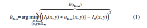
where S _nc is the set of pixels that do not belong to the class label “change” and which must be evaluated in the final change detection map. As first approximation for uˆ_b7→a, we can take for S _nc, the set of all pixels in the image. This can be justified because the area of change is usually quite small in proportion to the image which, also, can be considered (in a very first approximation) as noisy observations or outliers in the image data with which it is shown that the LSQ estimator performs well (especially thanks to the fact that the function E(u_b7→a) to be minimized is convex with regard to the parameter vector of the convolution filter u_b7→a). As a result, different efficient minimization procedures can be adopted [47].

In this work, we use a combination of conjugate gradient and a line minimization search routine guaranteeing a considerably increased convergence speed compared to other minimization methods. Another advantage of such a minimization technique consists on its ability to integrate some hard constraints on u_b7→a. In our case, since the two imaging modalities are circular invariant, we constraint u_{b→7 a} to be also circular invariant. To this end, at each iteration k of the conjugate gradient descent (CGD), we simply average each of the (sz × sz) parameter values of u^[_b^k_7→^] _a that are equidistant (in the L₁ distance sense) from the center of the convolution filter

Table 1: Heterogeneous datasets description No Dates Area Image size Event Satellite 1 Sept. 1995 – Jul. 1996 Sardinia, It 412×300 Lake overflow (30 m.) Landsat-5 (NIR band) / Optical 2 Nov. 1999 – Oct. 2000 Gloucester, Uk 330×590 Flooding (≈ 40 m.) SAR-ERS / Spot 3 July 2006 – July 2007 Gloucester, Uk 2325×4135 Flooding (0.65 m.) TerraSAR-X / QuickBird 2 4 Feb. 2009 – July 2013 Toulouse, Fr 4404×2604 Construction (2 m.) TerraSAR-X / Pleiades 5 May 2012 – July 2013 Toulouse, Fr 2000×2000 Construction (0.52 m.) Pleiades / WorldView 2 6 2001 – Jan. 2002 Congo, Af. 400×800 Nyiragongo volcano eruption (10 m.) Radarsat (3 / 5-looks) 7 June 2008 – June 2013 Island town, Chn. 415×403 Urbanization (8 m.) Radarsat-2 / Google Earth 8 June 2008 – Sept. 2012 Shuguang village, Chn 419×342 Building construction (8 m.) Radarsat-2 / Google Earth 9 June 2008 – June 2009 Yellow river, Chn. 409×367 River’s drying up (8 m.) Radarsat-2 (1 / 4-looks) 10 Aug. 2013 – Aug. 2015 Wehe river, Xi’an city, Chn. 392×303 flooding (2 m.) GF-1 (, bands) [46] 11 1999 – 2000 Gloucester, Uk 990×554 flooding (≈ 25 m.) SPOT/NDVI [17] 12 May 2002 – July 2009 Hubei Campus, Chn 240×240 Building construction (2.44 m.) QuickBird / IKONOS 13 April 2005 – July 2009 Wuhan University, Chn. 400×400 Building construction (3.28 m.) QuickBird / IKONOS

(see Algorithm 1). This allows us to integrate this constraint with a linear complexity with respect to the (sz × sz) parameters of the convolution filter. This overall minimization routine is presented in our basic model [1].

Algorithm 1 Concentric Circular Constraint

u(x,y)             Convolution filter of dim. (sz×sz) [input] u^◦(x,y)            Circular invariant filter [output] tab[x][y] 2D table (length,width)=(2sz,2) of floats

In order to improve this approximation of uˆ_b7→a, we can formulate the LSQ estimation problem of the convolution filter parameters as a fixed point problem involving a contraction mapping. Technically speaking, the first estimation of uˆ_b7→a allows us to obtain I_{b→7 a}(x,y) = I_b(x,y) ∗ u_b7→a(x,y), corresponding to the image preevent image projected on the modality of the post-event image. A simple pixel-by-pixel difference between I_{b→7 a}(x,y) and I_a(x,y) enables us then to produce an output image of absolute difference that is subsequently binarized to the “change” and the “non-change” class label. To this end, a Gaussian kernel is used to model the distribution of each class and the Expectation Maximization (EM) [48] algorithm is used both to estimate the parameters of this weighted distribution mixture but also to give an approximate estimate of S _nc (i.e., the pixels that does not belong to the class label “change”) with a binarization scheme in the Maximum Likelihood (ML) sense. This process allows us to finally better estimate uˆ_b7→a (see Eq. 1). This process is repeated until the stability of the algorithmic steady state fixed point thus defined is reached. This fixed point-based strategy yields to the following iterative procedure:

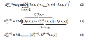
where S _nc^[0] stands for the whole image pixels and Φ^[_D^k+1] is the parameter vector of the two weighted normal kernels evaluated by the EM procedure (at iteration k + 1) on the difference image D(x,y).

ML_binarization{Φ^[_D^k+1],.} represents the binarization algorithm, based on Φ^[_D^k+1], in the Maximum Likelihood sense.

A second enhancement can be incorporated in this iterative procedure by simply inverting the direction of temporality of the two (before and after) satellite images in the algorithm introduced in our basic model [1]. Concretely, the estimation of uˆ_a7→b can be done by I_{a→7 b}(x,y) = I_a(x,y) ∗ u_{a→7 b}(x,y). This allows us to obtain another difference map between I_a7→b(x,y) and I_b(x,y). The reverse estimate can be used along with the original one to obtain an average estimate ensuring an improved (less noisy) difference image D(x,y) (see Algorithm 2).

In the case where the image before or after is a single-band image and the second image (possibly a multi-band) is then converted into gray levels and this pair of greyscale images are used as explained in Algorithm 3. A third improvement is proposed in the particular case where we have at our disposal two images before and after in colors (or with b > 1 color bands). In this case, the mapping and a difference map D(b, x,y) is estimated for each of the b images individually and sequentially. A difference map is defined finally as the L_∞ distance, for each pixel (x,y), between the b-components of each pixel (D(x,y) ← max_b D(b, x,y)) as illustrated in Algorithm 2.

After the fixed point becomes stable (concretely when S _nc^[k]≈

S _nc^[k+1], or after L_max^P , a maximal number of iterations is reached), the parameter vector of the Gaussian kernel mixture Φ_D (given by the EM procedure) is used to classify the difference map into two classes, once again, in the Sequential Maximum A Posteriori (SMAP) sense by using the multiscale, fine-to-coarse and coarse-tofine segmentation procedure [49].

This overall minimization routine is summarized in Algorithm 2 and in Algorithm 3 for a N-band image pair.

Algorithm 2 Convolution-Based Multimodal Change Detection

           S(x,y)       Binary change detection map [output]

           I_b(x,y)       The before image [input]

           I_a(x,y)       The after image [input]

           D(x,y)      Difference map

          Φ_D                  Vector parameters

EM

          L_max                  Maximal number of iterations for EM

         L_max^P                Maximal number of fixed-point iterations

1. Initialization

• Set S(x,y) with labels “no change” for each pixel

2. Fixed Point Estimation Step Repeat

• Estimate u_b7→a and u_a7→b (see [1])
• Circular constraint on u_b7→a and u_a7→b
• D(x,y) = |[I_b(x,y) ∗ u_b7→a(x,y)] − I_a(x,y)|

              .                    + |[I_a(x,y) ∗ u_a7→b(x,y)] − I_b(x,y)|

• Φ_D ← EM estimation (L_max^EM ) on D(x,y)
• S^[l] ← ML binarization of D(x,y) based on Φ_D
• k + +

        Until k<L_max^P            (orS(x,y)^[l],S(x,y)^[l−1]);

3. Segmentation Step

• S(x,y) ← SMAP on D(x,y) based on Φ_D

3. Experimental Results

3.1. Heterogeneous Dataset Description

Our strategy is validated by conducting a set of evaluation scenar-

ios on thirteen dissimilar heterogeneous datasets exhibiting different multi modality imaging data such as cross-sensor or multisensor (#1,#5,#12,#13), multisource (#2,#3,#4,#7,#8), multi-looking (#6,#9,#11) or multispectral images (#10)) with different resolution levels and image sizes and imaging a wide variety of changed events which are degraded by a wide variety of both noise type and levels as depicted in Table 1.

In all the experimental results, we recall that if one of the two images is in grayscale, we must convert the other image (colors or with b (> 1) bands) into grayscale to apply algorithm 2. Otherwise, if the two images contain the same number of bands (b), we rely on algorithm 3.

In addition, for computational reasons, we have reduced the image size so that the widest edge of it is at most equal to 500 pixels. For the estimation stage, the size sz of the convolutional (square) filter was set to 9, with a maximal iteration number L^G_max set to 200 and a fixed-point iteration number L_max^P equal to 2. The iteration

EM

number L_max used in the EM algorithm is 12 iterations (see our basic model [1]). For the segmentation stage, the depth of the SMAP was set to d=9 [49]. The regularization parameter θ was fixed to 0.9 (a value commonly used for this SMAP fine-to-coarse, coarse-to-fine segmentation algorithm [49, 54]).

Algorithm 3 CBMCD For N-Band Image pair

           S(x,y)         Binary change detection map [output]

          I_b(b, x,y)     The before image with b<N bands [input]

          I_a(b, x,y)      The after image with b<N bands [input]

           D(x,y)         Difference map

          Φ_D                     Vector parameters

          D(b, x,y)     Temporary map with b<N bands

EM

          L_max                      Maximal number of iterations for EM

         L_max^P                    Maximal number of fixed-point iterations

1. Initialization

• Set S(x,y) with labels “no change” for each pixel and fill D(k, x,y) with zeros

2. Fixed Point Estimation Step

Repeat for each band b of [I_b(b, x,y), I_a(b, x,y)] do

• Estimate ub7→a and ua7→b
• Circular constraint on u_b7→a and u_a7→b
• D(b, x,y)=|[I_b(b, x,y)∗u_b→7a]−I_a(b, x,y)|

                     .                   + |[I_a(b, x,y) ∗ u_a7→b] − I_b(b, x,y)|

D ← EM (L^EMmax iterations) on D(b, x,y)

• D(x,y) ← max_b D(b, x,y)
• S ← ML binarization of D(x,y) based on Φ_D
• k ← k + 1

        Until k<L_max^P            (orS(x,y)^[l],S(x,y)^[l−1]);

• Φ_D ← EM (L^EMmax iterations) on D(x,y)

3. Segmentation Step

• S(x,y) ← SMAP on D(x,y) based on Φ_D

3.2. Convolution Filter Estimation Step Result

For all the test scenarios, the maximum iteration number used in the conjugate gradient descent combined with the minimization line process, is sufficient to ensure the convergence of the minimization procedure. As example, we show, in Figure 1, how evolves the error rate along the minimization process. In addition, for all the scenarios, we estimate for u_b7→a or u_a7→b a convolution filter (that can be likened to a point spread function (PSF)) which is quite different from one dataset to another since the frequency response (or modulation transfer function) of the imaging modality is also quite different for each pair of imaging multi-modalities. Besides, the convolution filter size sz is also justified, enough because small values of parameters are estimated at the edges of the rectangular filter in all the tested cases (see Figure 2) for an example of convolution filter estimate).

3.3. Results & Evaluation

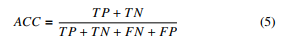
We evaluate and compare the obtained results using the classification rate accuracy that measures the correct changed and unchanged pixels percentages: ACC and the F-measure Fm which can be defined in the equations 5 and 6.

where TP and TN are the true positives and negatives. FN and FP designate the false negatives and positives.

Table 2 shows a comparison between our segmentation results and the different supervised and unsupervised state-of-the-art methods [9, 12, 16, 17, 20, 23]–[27, 32, 38, 51]–[53].

Figures 3, 4 and 5 compare qualitatively the obtained results. The average accuracy rate of our proposed model is higher than the supervised and unsupervised state-of-the-art methods, obtained by our proposed MCD model on the thirteen heterogeneous dataset is 87.78% with a F-measure equals to 0.444. Compared to these results, our preliminary model (non-circular invariant) [1] gave essentially the same result in terms of rate accuracy but with a much lower F-measure which did not exceed 0.389.

Globally, we notice that our approach works efficiently when a) the considered MCD problem tends towards the simple monomodal CD problem; in other words, in the case of a simple imaging modality which is not too different between the pre-event and post-event image (e.g., when there are similar sensors involving slightly different noise laws between the before and after images), or b) in the

case of a couple of images with high resolution, or c) in the case of

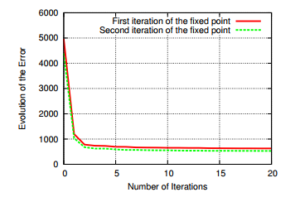
Figure 1: Cost function evolution (see Eq. (1) for the estimation of u_b7→a associated to dataset #1

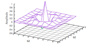
Figure 2: 9 × 9 Convolution filter estimate u_b7→a associated to dataset #1

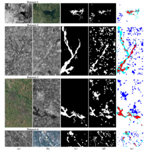
Figure 3: Multimodal datasets. (a) image t₁, (b) image t₂, (c) the ground truth; (d) binary map segmentation, (e) confusion map estimated by our model with white (TN), red (TP), blue (FP), cyan (FN) colors

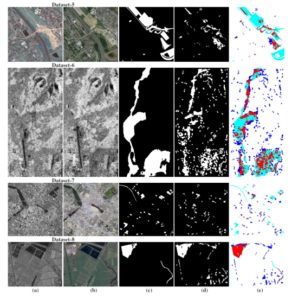
Figure 4: Multimodal datasets. (a) image t₁, (b) image t₂, (c) the ground truth; (d) binary map segmentation, (e) confusion map estimated by our model with white (TN),

red (TP), blue (FP), cyan (FN) colors

simple changed events images with a simple uniform texture; as example, a city is flooding by a river (inducing an uniform texture for a new zone or also in building construction or structure with a uniform texture very different from the rest of the image). Conversely, our approach is a little less suitable when it comes to processing a bi-temporal images in which the variability between the before and after images is more important. Otherwise said, in the case of an imaging modality resulting from the combination of active and passive sensors, thus inducing a combination of multiplicative and additive noises in the before and after images with a dissimilar noise law. Also for images pairs with a low spatial resolution and showing complex changed events; as example, urban site construction

(replacing a complex texture zone by the new complex texture area).

It requires about 54 seconds to the MCD to process an image.

The processing time depends on the estimation problem complexity, the size of image, and the mono or multichanel based estimation (or 660 seconds for the set of 13 image pairs considered in this validation study) using a code with non-optimized C++ version running on i7 − 930 Intel CPU with 2.8 GHz Linux machine.

4. Conclusion

We have presented in this work an efficient mapping model for the change detection problem in multimodal imagery relying on the parametric estimation of an invariant circular convolution CD model. Optimization of the model was performed on a convex quadratic error function using a conjugate gradient routine, whose optimal direction is determined by a quadratic line minimization algorithm, and formulated as a fixed point problem involving a contraction mapping. This allows us to project the before image in the imaging modality space of the second image and inversely so that a difference change map is then computed pixel by pixel and efficiently binarized with a multiscale Markov model. Our proposed strategy seems well suited for the multimodal change detection issue and robust enough against images provided under different resolution levels, type or level of noise and exhibiting a variety of natural event.

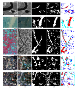
Figure 5: Multimodal datasets. (a) image t₁, (b) image t₂, (c) the ground truth; (d) binary map segmentation, (e) confusion map estimated by our model with white (TN), red (TP), blue (FP), cyan (FN) colors

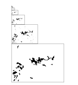
Figure 6: SMAP-based segmentation obtained for the dataset #1

Proposed model

0.896

Dataset [#1]	Accuracy rate
Proposed model	0.942

Dataset [#2]	Accuracy rate
Proposed model	0.835
Liu et al. [32]	0.818
Liu et al. [32]	0.655

Touati et al. [20]	0.949
Touati et al. [9]	0.932
Touati et al. [38]	0.943
Prendes et al. [26]	0.844

Touati et al. [38]	0.942
Zhang et al. [12]	0.975
PCC [12]	0.882

Correlation [26]

0.670

Mutual Information [26]

0.580

Table 2: Results comparison.

		Dataset [#3]		Accuracy rate
Dataset [#4]	Accuracy rate
Proposed model	0.882
Touati et al. [20]	0.867
Touati et al. [38]	0.878
Touati et al. [38]	0.881
Prendes et al. [50, 27]	0.918
Prendes et al. [25]	0.854
Copulas [23, 25]	0.760
Correlation [23, 25]	0.688
Mutual Information [23, 25]	0.768
Difference [51, 25]	0.782
Ratio [51, 25]	0.813

Dataset [#5]	Accuracy rate
Proposed model	0.866
Touati et al. [20] 0.853 Touati et al. [9] 0.870 Touati et al. [38] 0.877 Prendes et al. [26, 27] 0.844			Dataset [#6] Accuracy rate Proposed model 0.818 Chatelain et al. [24] 0.749 Correlation [24] 0.713 Ratio edge [24] 0.737	Dataset [#7] Accuracy rate Proposed method 0.946 zhan et al. [52] 0.979
Correlation [26, 27] 0.679 Mutual Information [26, 27] 0.759 Difference. [51, 27] 0.708 Ratio [51, 27] 0.661

Dataset [#8]	Accuracy rate
Proposed model	0.949
Touati et al. [38]	0.967
Liu et al. [16]	0.976
PCC [16]	0.821

Dataset [#9] Accuracy rate Proposed model 0.882 zhan et al. [52] 0.991	Dataset [#10] Accuracy rate	Dataset [#11] Accuracy rate Proposed model 0.882 HPT [17] 0.826
	Proposed model 0.862 zhan et al. [52] 0.937

	Dataset [#12]	Accuracy rate
	Proposed model	0.835
	Tang et al. [53]	0.986
	Multiscale [53]	0.991
Optical/Optical [#13]			Accuracy rate
Proposed model			0.815
Tang et al. [53]			0.959
Multiscale [53]			0.966

Acknowledgement

The authors thank the researchers whose shared the multi-modal dataset.

1. R. Touati, M. Mignotte, M. Dahmane, “Multimodal change detection using a convolution model-based mapping,” in eighth International Conference on Image Processing Theory, Tools and Applications, IPTA 2019, Istanbul, Turkey, November 2019, 2019, doi:10.1109/IPTA.2019.8936127.
2. N. Longbotham, F. Pacifici, T. Glenn, A. Zare, M. Volpi, D. Tuia, E. Christophe, J. Michel, J. Inglada, J. Chanussot, Q. Du, “Multi-Modal Change Detection, Application to the Detection of Flooded Areas: Outcome of the 2009-2010 Data Fusion Contest,” IEEE J. Sel. Topics Appl. Earth Observ., 5(1), 331–342, 2012, doi:10.1109/JSTARS.2011.2179638.
3. L. Su, M. Gong, P. Zhang, M. Zhang, J. Liu, H. Yang, “Deep Learning and Map- ping Based Ternary Change Detection for Information Unbalanced Images,” Pattern Recognition, 66(C), 213–228, 2017, doi:10.1016/j.patcog.2017.01.002.
4. R. Hedjam, M. Kalacska, M. Mignotte, H. Z. Nafchi, M. Cheriet, “Itera- tive Classifiers Combination Model for Change Detection in Remote Sensing Imagery,” IEEE Transactions on Geoscience and Remote Sensing, 54(12), 6997–7008, 2016, doi:10.1109/TGRS.2016.2593982.
5. R. Touati, M. Mignotte, “A multidimensional scaling optimization and fusion approach for the unsupervised change detection problem in remote sensing images,” in sixth IEEE International Conference on Image Processing Theory, Tools and Applications, IPTA’16, Oulu, Finland, December 2016, 1–6, 2016, doi:10.1109/IPTA.2016.7821021.
6. G. Liu, J. Delon, Y. Gousseau, F. Tupin, “Unsupervised change detection between multi-sensor high resolution satellite images,” in 24th European Sig- nal Processing Conference, EUSIPCO 2016, Budapest, Hungary, August 29 – September 2, 2016, 2435–2439, 2016, doi:10.1109/EUSIPCO.2016.7760686.
7. V. Alberga, “Similarity Measures of Remotely Sensed Multi-Sensor Images for Change Detection Applications,” Remote Sensing, 1(3), 122–143, 2009, doi:10.3390/rs1030122.
8. D. Brunner, G. Lemoine, L. Bruzzone, “Earthquake Damage Assessment of Buildings Using VHR Optical and SAR Imagery,” IEEE Transactions on Geo- science and Remote Sensing, 48(5), 2403–2420, 2010, doi:10.1109/TGRS. 2009.2038274.
9. R. Touati, M. Mignotte, M. Dahmane, “A new change detector in heteroge- neous remote sensing imagery,” in 7th IEEE International Conference on Image Processing Theory, Tools and Applications (IPTA 2017), Montreal, Canada, Qc, 2017, doi:10.1109/IPTA.2017.8310138.
10. G. Camps-Valls, L. Gomez-Chova, J. Munoz-Mari, J. L. Rojo-Alvarez, M. Martinez-Ramon, “Kernel-Based Framework for Multitemporal and Mul- tisource Remote Sensing Data Classification and Change Detection,” IEEE Trans. Geoscience and Remote Sensing, 46(6), 1822–1835, 2008, doi:10.1109/ TGRS.2008.916201.
11. P. Du, S. Liu, J. Xia, Y. Zhao, “Information Fusion Techniques for Change Detection from Multi-temporal Remote Sensing Images,” Inf. Fusion, 14(1), 19–27, 2013, doi:10.1016/j.inffus.2012.05.003.
12. P. Zhang, M. Gong, L. Su, J. Liu, Z. Li, “Change detection based on deep feature representation and mapping transformation for multi-spatial-resolution remote sensing images,” ISPRS Journal of Photogrammetry and Remote Sens- ing, 116, 24–41, 2016, doi:10.1016/j.isprsjprs.2016.02.013.
13. M. Gong, P. Zhang, L. Su, J. Liu, “Coupled Dictionary Learning for Change De- tection From Multisource Data,” IEEE Trans. Geoscience and Remote Sensing, 54(12), 7077–7091, 2016, doi:10.1109/TGRS.2016.2594952.
14. W. Zhao, Z. Wang, M. Gong, J. Liu, “Discriminative Feature Learning for Unsupervised Change Detection in Heterogeneous Images Based on a Cou- pled Neural Network,” IEEE Trans. Geoscience and Remote Sensing, 55(12), 7066–7080, 2017, doi:10.1109/TGRS.2017.2739800.
15. N. Merkle, P. F. S. Auer, R. Muller, “On the Possibility of Conditional Ad- versarial Networks for Multi-Sensor Image Matching,” in Proceedings of IGARSS 2017, IGARSS 2017, 1–4, Fort Worth, Texas, USA, 2017, doi: 10.1109/IGARSS.2017.8127535.
16. C. Wu, B. Du, L. Zhang, “Slow Feature Analysis for Change Detection in Mul- tispectral Imagery,” IEEE Transactions on Geoscience and Remote Sensing, 52(5), 2858–2874, 2014, doi:10.1109/TGRS.2013.2266673.
17. Z. G. Liu, G. Mercier, J. Dezert, Q. Pan, “Change Detection in Heterogeneous Remote Sensing Images Based on Multidimensional Evidential Reasoning,” IEEE Geoscience and Remote Sensing Letters, 11(1), 168–172, 2014, doi: 10.1109/LGRS.2013.2250908.
18. M. Volpi, G. Camps-Valls, D. Tuia, “Spectral alignment of multi-temporal cross-sensor images with automated kernel canonical correlation analysis,” ISPRS Journal of Photogrammetry and Remote Sensing, 107, 50–63, 2015, doi:10.1016/j.isprsjprs.2015.02.005.
19. X. Chen, J. Li, Y. Zhang, L. Tao, “Change Detection with Multi-Source Defec- tive Remote Sensing Images Based on Evidential Fusion,” ISPRS Annals of Photogrammetry, Remote Sensing and Spatial Information Sciences, 125–132, 2016, doi:10.5194/isprsannals-III-7-125-2016.
20. D. Tuia, D. Marcos, G. Camps-Valls, “Multi-temporal and Multi-source Remote Sensing Image Classification by Nonlinear Relative Normaliza- tion,” ISPRS Journal of Photogrammetry and Remote Sensing, 2016, doi: 10.1016/j.isprsjprs.2016.07.004.
21. Z. Liu, L. Zhang, G. Li, Y. He, “Change detection in heterogeneous remote sensing images based on the fusion of pixel transformation,” in 20th Interna- tional Conference on Information Fusion, FUSION 2017, Xi’an, China, July 10-13, 2017, 1–6, 2017, doi:10.23919/ICIF.2017.8009656.
22. L. T. Luppino, S. N. Anfinsen, G. Moser, R. Jenssen, F. M. Bianchi, S. B. Serpico, G. Mercier, “A Clustering Approach to Heterogeneous Change De- tection,” in Image Analysis – 20th Scandinavian Conference, SCIA 2017, Tromsø, Norway, June 12-14, 2017, Proceedings, Part II, 181–192, 2017, doi:10.1007/978-3-319-59129-2 16.
23. R. Touati, M. Mignotte, M. Dahmane, “Change detection in heterogeneous remote sensing images based on an imaging modality-invariant MDS represen- tation,” in 25th IEEE International Conference on Image Processing (ICIP’18), Athens, Greece, 2018, doi:10.1109/ICIP.2018.8451184.
24. L. T. Luppino, F. M. Bianchi, G. Moser, S. N. Anfinsen, “Remote sensing im- age regression for heterogeneous change detection,” CoRR, abs/1807.11766, 2018, doi:10.1109/MLSP.2018.8517033.
25. S. Benameur, M. Mignotte, J.-P. Soucy, J. Meunier, “Image restoration using functional and anatomical information fusion with application to SPECT-MRI images,” International Journal of Biomedical Imaging, 2009, 12 pages, 2009, doi:10.1155/2009/843160.
26. D. Kundur, D. Hatzinakos, “Blind image restoration via recursive filter- ing using deterministic constraints,” in Proc. International Conference on Acoustics, Speech, and Signal Processing, volume 4, 547–549, 1996, doi: 10.1109/ICASSP.1996.547737.
27. M. Mignotte, J. Meunier, “Unsupervised restoration of brain SPECT volumes,” in Vision Interfaces, VI’00, 55–60, Montre´al, Que´bec, Canada, 2000.
28. M. Mignotte, J. Meunier, “Blind deconvolution of SPECT images using a noise model estimation,” in SPIE Conference on Medical Imaging, volume 3979, 1370–1377, San Diego, CA, USA, 2000, doi:10.1117/12.387647.
29. M. Mignotte, J. Meunier, “Three-dimensional blind deconvolution of SPECT images,” IEEE trans. on Biomedical Engineering, 47(2), 274–281, 2000, doi: 10.1109/10.821781.
30. N. B. Smith, A. Webb, Introduction to Medical Imaging: Physics, Engineer- ing and Clinical Applications, Cambridge Texts in Biomedical Engineering, Cambridge University Press, 2010, doi:10.1017/CBO9780511760976.
31. T. Zhan, M. Gong, J. Liu, P. Zhang, “Iterative feature mapping network for detecting multiple changes in multi-source remote sensing images,” ISPRS Journal of Photogrammetry and Remote Sensing, 146, 38 – 51, 2018, doi: 10.1016/j.isprsjprs.2018.09.002.
32. W. H. Press, S. A. Teukolsky, W. T. Vetterling, B. P. Flannery, Numerical Recipes in C, Cambridge University Press, Cambridge, USA, 2nd edition, 1992.
33. C. Wu, B. Du, L. Zhang, “Slow Feature Analysis for Change Detection in Mul- tispectral Imagery,” IEEE Transactions on Geoscience and Remote Sensing, 52(5), 2858–2874, 2014, doi:10.1109/TGRS.2013.2266673.
34. Z. G. Liu, G. Mercier, J. Dezert, Q. Pan, “Change Detection in Heterogeneous Remote Sensing Images Based on Multidimensional Evidential Reasoning,” IEEE Geoscience and Remote Sensing Letters, 11(1), 168–172, 2014, doi: 10.1109/LGRS.2013.2250908.
35. M. Volpi, G. Camps-Valls, D. Tuia, “Spectral alignment of multi-temporal cross-sensor images with automated kernel canonical correlation analysis,” ISPRS Journal of Photogrammetry and Remote Sensing, 107, 50–63, 2015, doi:10.1016/j.isprsjprs.2015.02.005.
36. A. Dempster, N. Laird, D. Rubin, “Maximum likelihood from incomplete data via the EM algorithm,” Royal Statistical Society, 1–38, 1976, doi: 10.1111/j.2517-6161.1977.tb01600.x.
37. C. Bouman, M. Shapiro, “A Multiscale Random Field Model for Bayesian Image Segmentation,” IEEE Trans. on Image Processing, 3(2), 162–177, 1994, doi:10.1109/83.277898.
38. J. Prendes, M. Chabert, F. Pascal, A. Giros, J.-Y. Tourneret, “Change detection for optical and radar images using a Bayesian nonparametric model coupled with a Markov random field,” in Proc. IEEE International Conference on Acous- tic, Speech, and Signal Processing, ICASSP’15, Brisbane, Australia, 2015, doi:10.1109/ICASSP.2015.7178223.
39. O. D. Team, “The ORFEO Toolbox Software Guide,” 2014, available at http://orfeo-toolbox.org/.
40. T. Zhan, M. Gong, J. Liu, P. Zhang, “Iterative feature mapping network for detecting multiple changes in multi-source remote sensing images,” ISPRS Journal of Photogrammetry and Remote Sensing, 146, 38–51, 2018, doi: 10.1016/j.isprsjprs.2018.09.002.
41. Y. Tang, L. Zhang, “Urban Change Analysis with Multi-Sensor Multispectral Imagery,” Remote Sensing, 9(3), 2017, doi:10.3390/rs9030252.
42. M. Mignotte, C. Collet, P. Pe´rez, P. Bouthemy, “Sonar image segmentation using an unsupervised hierarchical MRF model,” IEEE Trans. on Image Pro- cessing, 9(7), 1216–1231, 2000, doi:10.1109/83.847834.
43. M. Mignotte, J. Meunier, “Blind deconvolution of SPECT images using a noise model estimation,” in SPIE Conference on Medical Imaging, volume 3979, 1370–1377, San Diego, CA, USA, 2000, doi:10.1117/12.387647.
44. M. Mignotte, J. Meunier, “Three-dimensional blind deconvolution of SPECT images,” IEEE trans. on Biomedical Engineering, 47(2), 274–281, 2000, doi: 10.1109/10.821781.
45. N. B. Smith, A. Webb, Introduction to Medical Imaging: Physics, Engineer- ing and Clinical Applications, Cambridge Texts in Biomedical Engineering, Cambridge University Press, 2010, doi:10.1017/CBO9780511760976.
46. T. Zhan, M. Gong, J. Liu, P. Zhang, “Iterative feature mapping network for detecting multiple changes in multi-source remote sensing images,” ISPRS Journal of Photogrammetry and Remote Sensing, 146, 38 – 51, 2018, doi: 10.1016/j.isprsjprs.2018.09.002.
47. W. H. Press, S. A. Teukolsky, W. T. Vetterling, B. P. Flannery, Numerical Recipes in C, Cambridge University Press, Cambridge, USA, 2nd edition, 1992.
48. A. Dempster, N. Laird, D. Rubin, “Maximum likelihood from incomplete data via the EM algorithm,” Royal Statistical Society, 1–38, 1976, doi: 10.1111/j.2517-6161.1977.tb01600.x.
49. C. Bouman, M. Shapiro, “A Multiscale Random Field Model for Bayesian Image Segmentation,” IEEE Trans. on Image Processing, 3(2), 162–177, 1994, doi:10.1109/83.277898.
50. J. Prendes, M. Chabert, F. Pascal, A. Giros, J.-Y. Tourneret, “Change detection for optical and radar images using a Bayesian nonparametric model coupled with a Markov random field,” in Proc. IEEE International Conference on Acous- tic, Speech, and Signal Processing, ICASSP’15, Brisbane, Australia, 2015, doi:10.1109/ICASSP.2015.7178223.
51. O. D. Team, “The ORFEO Toolbox Software Guide,” 2014, available at http://orfeo-toolbox.org/.
52. T. Zhan, M. Gong, J. Liu, P. Zhang, “Iterative feature mapping network for detecting multiple changes in multi-source remote sensing images,” ISPRS Journal of Photogrammetry and Remote Sensing, 146, 38–51, 2018, doi: 10.1016/j.isprsjprs.2018.09.002.
53. Y. Tang, L. Zhang, “Urban Change Analysis with Multi-Sensor Multispectral Imagery,” Remote Sensing, 9(3), 2017, doi:10.3390/rs9030252.
54. M. Mignotte, C. Collet, P. Pe´rez, P. Bouthemy, “Sonar image segmentation using an unsupervised hierarchical MRF model,” IEEE Trans. on Image Pro- cessing, 9(7), 1216–1231, 2000, doi:10.1109/83.847834.

(Click Here)

(Click Here)