1. Introduction

Dengue Fever (DF) outbreak happened annually, but every year the number of victims is very high. In the present decade, Ketharpal mentioned that dengue is endemic to 128 countries, mostly developing nations, posing a risk of death to approximately 3.97 billion people annually [1]. Cartographic approaches estimated that 390 million dengue infections annually, out of which 96 million cases evident apparently [2,3]. World health organization (WHO) stated that more than 70% of the population at risk for dengue worldwide live in member states of the WHO South-East Asia Region and Western Pacific Region [4]. WHO categorized the variable endemicity of dengue fever into four categories. Indonesia is included in category A which means the endemic occurs due significant public health problem, a leading cause of hospitalization and death among children, hyperendemicity with all four serotypes circulating in urban areas, and spreading to rural areas [5].

More than thirty-nine thousand (39,876) DF cases and 254 deaths were reported by Indonesian Health Ministry from January to March 2020 [6,7,8]. For significant reduction of dengue mortality, the strategies for the prevention of dengue include prompt diagnosis of fever cases, providing appro­priate clinical management, and controlling vector, and personal protection methods. Therefore, severe cases can be managed with appropriate treatment, and health personnel at all level can be trained. Improved outbreak prediction and detection through coordinated surveillance will be able to reduce DF spread and effected area [9, 10].

Many types of research have been done in predicting the spread and DF affected area. A five years dataset from Sleman, a district in Central Java Indonesia are used for predicting the spread of the DF [11]. Mahdiana’s model is based on vector autoregressive spatial autocorrelation (varsa). A four years dataset from Bandung stated that the incidence rate of dengue fever was not related to annual rainfall, population density, larva free index, and prevention Program [12]. The spreading of DF in Surabaya, Indonesia, is modelled using statistical learning [13,14]. Besides of statistical learning approach, many researchers also developed the model in the machine learning approach. Various machine learning algorithms are compared, such as naive Bayes, random forests, minimal sequential optimization [15]. They collected data from the health department, Karuna medical hospital, Kerala, and online sources. The authors stated random forests gives better accuracy for the early detection of dengue disease.

On the other hand, the use of neural networks as an algorithm for predicting disease has been widely used. An artificial neural network is used to predict the DF outbreak in Srilanka [16], using similar approach [17,18] the DF outbreak in Thailand modelled and in the Northwest Coast of Yucatan, Mexico and San Juan, Puerto Rico, respectively. Most of the artificial neural network that has been used to develop the model is multi-layer perceptron, with the input as the population characteristics in each region and number of DF infected in the previous years for predicting the number of DF infected in the current or next year.

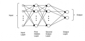
Figure 1.  Multi-Layer Perceptron Neural Network

In this research, we proposed a spatial multi-layer perceptron model for predicting the DF outbreak. As a case study, we used DF data in Surabaya. The proposed model adopts the spatial approach in statistical learning as well as the multi-layer perceptron in the machine learning approach. This proposed model tries to accommodate the nature of DF disease spreading. Because DF is a type of disease that spreads through dengue mosquitoes, if DF infects a particular area, the surrounding areas will be vulnerable to the spread of the disease (spatially correlated). Therefore, disease prediction in a particular area is greatly influenced by the DF disease in the surrounding area. So, to predict the possibility of the spread of dengue fever in a particular area, we need to calculate the spread DF data from the surrounding areas. This data will be calculated separately for each region (spatial dependent). This proposed model will implement in Multi-Layer Perceptron Model (MLP) Neural Network. The MLP NN model does not accommodate the spatial dependency in the neural-network construction. This proposed model tries to build a spatial MLP model to accommodate the nature of DF decease spreading.

Additionally, we also present the model for predicting the DF web basely. Since currently, the data for DF victims is manually collected at community health centers, and it will be reported to the regional health department. Based on this DF data, the city and province will take a curative and preventive action to prevent DF outbreak in next year. Urgent measures also being taken by community health centers during outbreaks such as fogging or spreading abate powder in water collecting area.  Without a sound information system on DF outbreak location and spreading, the government cannot control and minimize dengue mortality.

2. Research Methods

2.1. Multilayer Perceptron

 Multilayer perceptron (MLP), also often called as feed­for­ward neural networks consists of neurons that are ordered into layers (Figure 1). The first layer is called the input layer, and the last one is called as the output layer, the layers between are hidden layers [19].

The main goal of MLP is to approximate some function ; e.g. in a regression,  ; the function  maps the input vector  into the a value . The feedforward network defines a mapping  and learns the value of the parameters  that result in the best function approximation.

In the general MLP (Figure 1), we know that each layer can be modelled as a function of

where  is the activation function,  are weights in the layer,  is the input vector, which can also be the output of the previous layer, and  is the bias vector. The hidden layers, which are located in between the input and the output of a neural network, will perform nonlinear transformations of the input in the network. The number of the hidden layers are varied. It depends of the function of the neural network. Similarly, the number of the layers may vary. It depends on their associate weights [20].

The function f is called the transfer function. The transfer function used in this research is ReLu (Rectified Linear Unit) [21]. This function is defined as . Visually it can be seen in Figure 2.

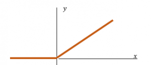
Figure 2. Rectified Linear Unit

2.2 Spatial Multilayer Perceptron

It is well known that the dengue fever happening most in tropical countries and considered as the fastest spreading mosquito-borne disease. It is transmitted by Aedes mosquito which infected with a dengue virus. The spreading of this diseases is spatially correlated [13]. The MLP model does not accommodate the spatial dependent in the neural-network construction. There­fore, in this paper we modi­fied the Multilayer Perceptron Model (MLP), to accommo­date the spatial nature of the disease.

In this model, we assumed that the spread of the diseases is in the first-order contiguity level. That is, the number of cases in location  is contagious to its north, east, south, and west neigh­borhoods. Some additional explanatory variables are also included in the model. They are sex ratio, poverty percentage, population density. In this proposed model, the first layer equation can be written as follows:

where:

	:	Number of cases in the location
	:	The th neuron weight w.r.t explanatory variable
	:	The explanatory variable  in the location
	:	The -th neuron weight w.r.t response variable  in the location
	:	Number of dengue fever cases in the location
	:	The  (north, east, south, west) location of the location
	:	Bias
	:	Number of explanatory variables ( )
	:	Number of neurons
	:	index

In this model the input of the MLP is changed depend on the location .  To give an illustration, let predicts the number of cases in sub-district Balongsari (Figure 3). This region shares borders to sub-district Asemrowo (north), sub-district Tanjung­sari (east), sub-district Lontar (south) and sub-district Manukan Kulon (west).

	(A) Asemrowo
(M) Manukan Kulon	(B) Balongsari	(T) Tanjungsari
	(L) Lontar

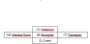
Figure 3: Sub-district Balongsari surrounding area

So, the model can be written as

here  is the sex ratio in Balongsari,  is the poverty percentage in Balongsari,  is the population density in Balongsari.   and  are the number of DF case in Asemrowo, Tanjungsari, Lontar and Manukan Kulon respectively. The input neurons of the model adaptively changes with respect to the region .

2.3 Design Spatial Multi-Layer Perceptron Neural Network

The design uses seven neurons; three neurons represent sex ratio, percentage of poverty and population density of each region under health community center s recorded in 2018. The other four neurons are dynamic neurons. They represent the number of cases in the north, east, south, and west. These neurons depend on the location s (See Figure 4).

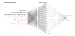
Figure 4: Ilustration for sub-district Balongsari

We used 252 data training (data from 2012-2015) and 126 (data from 2017-2018) data testing. The training process used 3500 epochs (Table 1), and mean squared error is used to measure the loss/error function and we used the stochastic gradient descent as the optimizer.

After some modeling the best design for this case used 1 hidden layer with 17 neurons and 1 output layer (Table 2). The activation function is rectified linear unit (Relu) on the hidden layer and linear on the output layer (Figure 5). This model is implemented as Python functions. It can be used to the other regions as far as the dataset is provided.

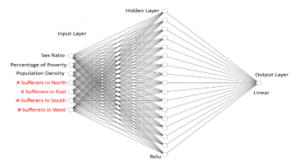
Figure 5: The design of spatial MLP model

Table 1: Setting the Number of Epochs and Neuron

Model	Epochs	Neuron	Loss on Data Training	Loss on Data Validation
1	1500	15	0.0198	0.0403
2		17	0.0187	0.0407
3		20	0.0196	0.039
4		22	0.0182	0.039
5	3500	15	0.0189	0.0304
6		17	0.0176	0.0294
7		20	0.0184	0.0383
8		22	0.0171	0.0399
9	4000	15	0.0184	0.0309
10		17	0.0171	0.0304
11		20	0.0181	0.0381
12		22	0.0169	0.0302

Table 2: Setting the Hidden Layer

Model	Layer	#Neuron Hidden Layer 1	# Neuron Hidden Layer 2	Loss on Data Training	Loss on Data Validation
1 hidden	1	17	–	0.0176	0.0294
2 hidden	2	17	7	0.0181	0.0297

3. Result and Discussion

3.1. Data Collection

Data we collected from Surabaya city consist of weather and population characteristic data. Weather data records the num­ber of rainy days in a year, precipitation, maximum and mini­mum temperature, maximum and minimum humidity. The result shows that Surabaya weather is not significantly different, so it will not be used as the model’s explanatory factor. Population charac­te­ris­tic data will be used in the model, and they are sex ratio, popu­la­tion density, and poverty percentage.

3.2. Data Training and Testing

We use the recorded data from 2012-2015 as the training dataset and the data from 2016 to validate the model. The training dataset consists of 63×4 = 252 data. As usual, we normalized the data set in advanced. The loss of the training data is 0.0176. Figure 5 shows the fitting of the real data to the prediction one. The horizontal axe represents the community health center, the vertical axe represents the number of cases in each community health center, recorded from 2012-2015. Figure 6 shows that the prediction can follow the pattern of the real dataset. During 2012-2013 the number of cases was high, and it started to drop in 2014-2015. The box plot of the data training (Figure 7) shows that there are several outliers in the real dataset and those outliers cannot be captured by the proposed model. The median of the prediction is not signi­ficantly different from the real one, but the interquartile range of the prediction is smaller than the real dataset. The two-samples t-test for the training data set is summarized in Table 4 The one-sided p-value is 0.335, we can conclude that there is no mean difference between the real dataset and the predicted one. The mean difference is -0.53 and the 95% confidence interval of the mean difference is (-2.96, 1.91).

Table 3: Surabaya Statistics in 2018

	Min	Mean	Max
Population (thousand)	12541	45802	87561
Area (Km2)	0.915	2.001	14.400
Density (thousand/Km2)	2733	46992	541022
Sex Ratio (Men/Women)	91.5	99.27	110.93
Poverty percentage (%)	4.03	18.02	55.46
Rainy day (days/month)	9.83	13.99	16.00
Precipitation (mm/month)	129.9	164.6	194.9
Max Humidity per month	70	88.72	94.75
Min Humidity per month	46.08	53.14	57.83
Max Temperature	28.21	33.30	34.43
Min Temperature	23.11	26.29	28.73

Table 4: Two-samples t-test for Data Training

	Real	Predicted
Mean	18.86508	19.39285714
Variance	262.0455	125.4745304
Observations	252	252
Hypothesized Mean Difference	0
df	447
t Stat	-0.425602637
P(T<=t) one-tail	0.335301126
t Critical one-tail	1.648269625
P(T<=t) two-tail	0.670602253
t Critical two-tail	1.965285234

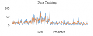
Figure 6: The real and prediction line chart of data training from 2012-2015.

We use the recorded data from 2017-2018. There are 126 data. Applying the modelled, the loss value of the testing dataset is 0.052. Some of the prediction are lower/higher than the reality (see Figure 8). Some community health centers reported that there were no dengue fever cases in their area (the number of cases equal to zero), but in their surrounded areas reported highly dengue fever cases. As the result, the real zero number cannot be captured as zero in the model. The model will predict the number of infected in that area as the mean value of the neighborhood. This situation is acceptable, since the predicted number will give early warning to that region to prevent the outbreak in that area.

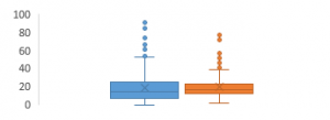
Figure 7: Box plot of the training dataset

3.3. Discussion

In this study, we prosed a spatial-MLP model, which accommo­date the spatial property of the dataset. Comparing the other NN models which are used by [16,17,18,19,20] this model uses dynamic variables, which depend on the neighborhood of a region as well as the external variables. The model by [16,17,18,19,20] used only external variables, which do not depend on the neighborhood of a region.

The same dataset has been modelled using the Geostatistical Weighted Regression (GWR) [13]. In [13], the predicted model can follow the pattern of the actual dataset. However, the MSE of the prediction for the years 2017-2018 is 8.59. Compare to this model, the mean square error of the testing data set in the same years is lower, that is 8.07. The t-test shows that there is no significant difference between the mean of the real and the mean of predicted of the testing dataset (Table 5). This model is better than the GWR. However, the computation time of GWR is faster than the spatial-MLP. Since in the spatial-MLP, we have to do the hyper­para­meter tuning for finding the best model. This model has limitation. It cannot capture the zero in the dataset. The zeros will be predicted as the mean values of the surrounding areas. In this study we prosed a spatial-MLP model, which accommo­date the spatial property of the dataset. Comparing the other NN models which are used by [16,17,18] this model uses dynamic variables, which depend on the neighborhood of a region as well as the external variables. The model by [16,17,18] used only external variables, which are not depend on the neighborhood of a region.

The same dataset has been modelled using the Geostatistical Weighted Regression (GWR) [13]. In [13], the predicted model can follow the pattern of the true dataset. However, the MSE of the prediction for the years 2017-2018 is 8.59. Compare to this model, the mean square error of the testing data set in the same years is lower, that is 8.07. The t-test shows that there is no significant difference between the mean of the real and the mean of predicted of the testing dataset (Table 5). This model is better than the GWR. However, the computation time of GWR is faster than the spatial-MLP. Since in the spatial-MLP, we have to do the hyper­para­meter tuning for finding the best model. This model has limitation. It cannot capture the zero in the dataset. The zeros will be predicted as the mean values of the surrounding areas.

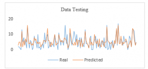
Figure 8: The real and prediction line chart of data training from 2017-2018.

Table 5: Two-samples t-test for Data Testing

	Real	Predicted
Mean	5.126984	5.428571
Variance	16.01575	10.10286
Observations	126	126
Hypothesized Mean Difference	0
df	238
t Stat	-0.6624
P(T<=t) one-tail	0.254176
t Critical one-tail	1.651281
P(T<=t) two-tail	0.508353
t Critical two-tail	1.969982

3.4 Web implementation

This modeled is implemented in a website base to help the “Dinas Kesehatan Surabaya” (The Surabaya Public Health Department) monitoring the dengue fever outbreak. From this website, users can see DF spreading data for each district in Surabaya in the selected year (Figure 9). Data on the number of victims in each sub-district will be displayed in red, yellow and green, with red representing the largest number of victims and green representing the smallest number of victims. Users can spe­cify the upper limit of each color representative. The appli­cation will then automatically determine the color gradation based on the input, so that the user can see number of victims in each sub-district that representing in color information. The legend from this gradation color information will display next to the map. User also could choose and see detail information from each sub-district and number of DF victims.

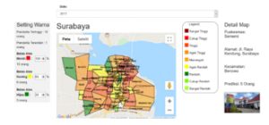
Figure 9: The web design for implemented model

Users can also see details of the number of patients in each sub-district and compare the movement of the number of patients in 3 years presented in tabular form (Figure 10). This data also can be viewed in graphical form (Figure 11).

This visual information will provide more informative information to help The Surabaya Public Health Department monitoring and prevent the dengue fever outbreak for each sub-district.

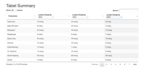
Figure 10: Summarize comparizon spreading DF disease data for each sub-district in Surabaya

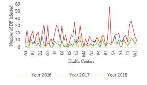
Figure 11: Summarize comparizon spreading DF disease data for each sub-district in Surabaya

4. Conclusion

In this paper we proposed spatial multi-layer perceptron (spatial MLP) model for predicting dengue fever in Surabaya. The model can capture the data pattern. Additionally, the model is implemented in the web-based database. The Surabaya Public Health Department (Dinas Kesehatan Surabaya) can input the data and predict the outbreak online. However, right now in some regions the predictions are not performed well, especially when that region has zero value. The zeros will be predicted as the mean values it’s neighborhood. In the next research, we will expand the model into spatial-temporal multi-layer perceptron (spatial-temporal MLP) model, which can capture data dependencies not only spatially, but also temporally.

Acknowledgement

The authors would like to express their gratitude to the reviewers’ feedbacks which certainly improve the clarity of this paper. We also would like to thank to Surabaya Public Health Office (Dinas Kesehatan Surabaya), for the fruitfull discus­sions. Thanks to Holiyed Hadi for the fruitful discussion on the data base web-design construction. This research is funded by the Ministry of Research, Technology, and Higher Edu­ca­tion Republic of Indonesia and the Petra Christian University Institute of Research and Community Outreach.

1. N. Khetarpal N, I. Khanna, “Dengue fever: causes, complications, and vaccine strategies”, Journal of Immunology Research, 2016, 1-14, 2016, doi.org/10.1155/2016/6803098
2. S. Bhatt, P.W. Gething, O.J. Brady, J.P. Messina, A.W. Farlow, Moyes CL, J.M. Drake, J.S. Brownstein, A.G. Hoen, O. Sankoh, M.F. Myers, D.B. George, T. Jaenisch , G.R.W. Wint, C.P. Simmons, T.W. Scott, J.J. Farrar, S.I. Hay, “The global distribution and burden of dengue”, Nature, 496 (7446), 504–507, 2013, doi: 10.1038/nature12060
3. O.J. Brady, P.W. Gething, S. Bhatt, J.P Messina, J.S. Brownstein, A.G. Hoen, C.L. Moyes, A.W. Farlow, T.W. Scott, S.I., Hay SI, “Refining the global spatial limits of dengue virus transmission by evidence-based consensus”, PLoS Neglected Tropical Diseases, 6 (8), 1-15, 2012, doi.org/10.1371/journal.pntd.0001760
4. WHO, “Dengue guidelines or diagnosis, treatment, prevention and control”, World Health Organization, 2009
5. WHO, “Comprehensive Guidelines for prevention and control of dengue and dengue haemorrhagic fever”, World Health Organization- Regional Office for South-East Asia, World Health Organization, 2011.
6. Tempo, “Dengue fever claims 254 Indonesian lives amid COVID-19 Outbreak”, 7 April 2020. Retreived from
   https://en.tempo.co/read/1328820/dengue-fever-claims-254-indonesian-lives-amid-covid-19-outbreak, accessed on 5 May 2020
7. Kompas, “Higher than corona, dengue cases reach 17,820 Indonesia”. 11 Maret 2020. Retreived from
   https://nasional.kompas.com/read/2020/03/11/17091361/lebih-tinggi-dari-corona-kasus-dbd-tembus-17820-se-indonesia, accessed on 5 April 2020
8. Kompas, “Increase rapidly, 2016 cases of dengue fever in East Java, 20 died” 13 Maret 2020. Retrieved from
   https://surabaya.kompas.com/read/2020/03/13/22200881/bertambah-2016-kasus-dbd-di-jatim-20-meninggal, access on 10 April 2020.
9. WHO, “Global strategy for dengue prevention and control 2012-2020”, World Health Organization, 2012.
10. W. Wen-Hung, N.U. Aspiro, R.C. Max, A. Wanchai, L. Po-Liang, C. Yen-Hsu, Sheng-Fan, “Dengue hemorrhagic fever a systemic literature review of current perspectives on pathogenesis, prevention and control”, Journal of Microbiology, Immunology and Infection, Article in Press. 2020
11.  D. Mahdiana, E. Winarko, A. Ashari, H. Kusnanto, “A model for forecasting the number of cases and distribution pattern of dengue hemorrhagic fever in Indonesia” International Journal of Advanced Computer Science and Applications, 8(11): 143-150, 2017, DOI:10.14569/IJACSA.2017.081118
12. K. Anggia, S.Y.I. Sari, H.U. Sumardi, E.P. Setiawati, “Incidence of dengue hemorrhagic fever related to annual rainfall, population density, larval free index and prevention program in Bandung 2008 to 2011”, Althea Medical Journal, 2(2), 262-267, 2015.
13. S. Halim, T. Octavia, Felecia, A. Handojo, “Dengue fever outbreak prediction in Surabaya using a geographically weighted Regression”. Times-Icon Proceeding, 2019, DOI: 10.1109/TIMES-iCON47539.2019.9024438
14. S. Halim, Felecia, T. Octavia, “Statistical learning for predicting dengue fever rate in Surabaya”, Jurnal Teknik Industri, 22(1), 37-45, 2020, doi.org/10.9744/jti.22.1.37-46
15. N. Rajathi, S. Kanagaraj, R. Brahmanambika, K. Manjubarkavi, “Early detection of dengue using machine learning algorithms” International Journal of Pure and Applied Mathematics, 118(18), 3881-3887, 2018.
16. P.H.M.N. Herath, A.A.I. Perera, H.P. Wijekoon, “Prediction of dengue outbreaks in Srilanka using artificial neural network”, International Journal of Computer Applications, 101, 1-5, 2014, doi:10.1.1.735.9487
17. B. Jongmuenwai, S. Lowanichchai, S. Jabjone, “Prediction model of dengue hemorrhagic fever outbreak using artificial neural networks in Northeast of Thailand”, International Journal of Pure and Applied Mathematics, 118(8), 3407-3417, 2018.
18. A.E. Laureano-Rosario, A.P. Duncan, P.A. Mendez-Lazaro, J.E. Garcia-Rejon, S. Gomez-Carro, J. Farfan-Ale, D.A. Savic, F.E. Muller-Karger, “Application of artificial neural networks for dengue fever outbreak predictions in the Northwest Coast of Yucatan, Mexico and San Juan, Puerto Rico”, Tropical Medicine Infectious Disease, 3(5), 1-16, 2018, doi:10.3390/tropicalmed3010005
19. D. Svozil, V. Kvasnicka, J. Pospichal, “Introduction to multi-layer feed-forward neural networks”, Chemometrics and Intelligent Laboratory Systems,39,43-62, 1997, doi.org/10.1016/S0169-7439(97)00061-0
20. R. Collobert, S. Bengio, “Links between perceptrons, MLPs and SVMs”, Proceeding of International Conference on Machine Learning (ICML), 2004, doi.org/10.1145/1015330.1015415
21. L. Yann, Y. Bengio, H. Geoffrey, “Deep learning”, Nature, 521(7553), 436-444, 2015.

(Click Here)

(Click Here)