1. Introduction

The digital sensing and processing based on the Nyquist criteria made a tremendous impact on real-time applications. The scale of data accumulated by digital conversion has increased from a few to exponential growth. In many emerging applications it will be very complex to store and transmit over the communication channel. Therefore, it is very much essential to find out an alternative for the Nyquist criteria which can reconstruct the signals with few numbers of samples than the Nyquist criteria. The Compressive Sensing theory (CS) [1-7], which is an asymmetric concept [8] with the simple decoder and dumb encoder, can reconstruct the sparse signals when the samples are acquired other than the Nyquist criteria.

The signal acquisition in CS theory is the product of random measurement matrix  and analog signal  leads to CS measurements  [9, 10] defined by equation (1).

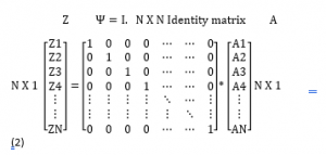
The Nyquist criterion as shown in equation (2), is extended to illustrate compressive theory, where is an analog signal,  is unity (identity) matrix of size  and  is the Nyquist samples. In CS unity matrix is replaced with a random matrix such as Bernoulli Matrix [11], Uniform Spherical, Partial Hadmard, etc. Samples that are obtained by multiplying the analog signal with the random matrix are called CS measurements  as shown in equation (3).

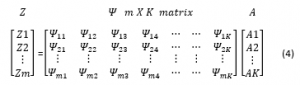
These CS measurements are related to only sparse (big amplitude) signal, that’s why is less than . Random matrix is modified as shown in equation (4) by including only those columns related to sparsity. Remaining signals  are not processed which may be located anywhere in the signal. Therefore, CS is an asymmetric theory.

Various Matching Pursuit algorithms [12] are used to solve the linear equation (4). Orthogonal Matching Pursuit (OMP) is compatible for sparse recovery [13-15]. This OMP will search the sparse related columns iteratively which appears in the random matrix. These are the best approximate-correlated columns that correspond to the sparse signal. One best-correlated column is searched in the iterations and removed from the random matrix. Like this finally updated matrix  of dimension  is obtained. The sparse reconstructed signal is obtained by solving the Least Square Problem (LSP). The complete OMP procedure is bellowed:

1. Declaration: Declare residual matrices , ,  and the index set . Initialize iteration to 1.
2. Search Index: Search the most correlated index by solving the optimization problems and generate and
3. Residual Status Update: Revise the index set and estimate the residual.

4. Iterations: and go back to search index step suppose .
5. LSP: Least Square problem, Find the inverse corresponding   to get reconstructed sparse signal

Further write up of the paper is as follows. 2 briefs design methodology. In 3 VLSI architecture is proposed. The results of the work are shown in 4. Finally, work is concluded with future work in 5.

2. Design Methodology

2.1. OMP (Reconstruction Algorithm) Blocks

OMP is a sequential algorithm (as shown in Figure1) where the Optimization block is formed by combining the Search Index and Residual update. CS measurements  which are in HEX format , Random Matrix  of dimensions  and sparsity count  are applied as inputs. Correlated columns  related sparse signals are identified. From these correlated columns, reconstructed signal  is calculated by taking the inverse of the matrix as shown in equation (5) and (6) in LSP.

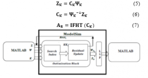
Figure 1: OMP Blocks

2.2. Input for OMP Architecture

MATLAB tool is used to generate input for OMP Architecture. The unsigned gray image of any dimensions is resized into to . Double Precision format for processing purposes and integer format for display purpose is followed. Since the image does not exhibit sparsity property in the normal domain so it is converted into FHT (Foreward Hadmard Domain). Less magnitude coefficient values are treated as zero by selecting a proper threshold value. This is asymmetric contrast to the Nyquist criteria. These zero value signals may be located anywhere in the image. These are converted to in HEX number and stored as a text file which is used as input for OMP VLSI Architecture. The complete procedure of creating a text file is shown in Figure2.

Figure 2: Text File Creation Flow

3. Proposed VLSI Architecture

The text file which is obtained from the previous step and the random matrix are stored in different RAM in the proposed OMP architecture as shown in Figure3. The tree structure (Wallace tree) as shown in Figure4 is used to obtain the inner product vector. The CS measurements in the form of   dimensions are applied to the Wallace tree along with random variables.

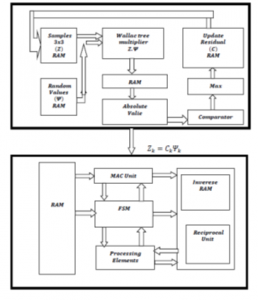
Figure 3: Proposed OMP Architecture

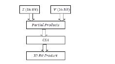
Figure 4: Multiplier (Wallace Tree)

In this proposed architecture, a carry-save adder (CSA) as shown in Figure5 is used to perform the fast addition of partial products. At the beginning of the calculations, the accumulator register is reset to zero. Then, the first partial product,  , is selected by the multiplexer and applied to the  -bit adder. The other input of the adder comes from the  -bit register. Hence, at this stage, the output of the  -bit adder will be  = =P. With the upcoming clock tick, this will be stored in the accumulator register. Next, the second partial product, Q, will be chosen by the multiplexer. This will be added to the current value of the  -bit register which gives . This procedure will be repeated for the remaining partial products. With each clock tick, a new partial product will be added and the result will be stored in the  -bit register. The control unit is used to generate an appropriate signal for the select input of the multiplexer. Speed up of the -bit adder is achieved by implanting a carry-lookahead structure for a -bit adder.

Figure 5: Carry save Adder

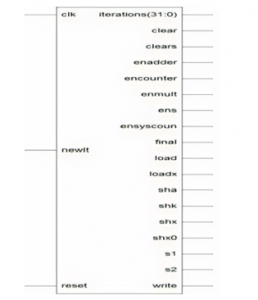
Figure 6: Control Path Block

In a single clock cycle, it cannot be completed since the carry bit has to propagate. CSA is required in different stages of the OMP algorithm. This adder architecture is critical as it is used for many numbers of operations. The complexity of the adder depends on the operation like subtraction, multiplication, and division. In general carry-save adders connected in a tree-like structure can reduce the number of operations from  to  compare to parallel adders. This in turn contributes to reconstruction time. Within the tree structure, an adder is designed using    multiplexers which can reduce the delay of higher multiplexers and it address reconstruction time. Once the product vector is obtained from the tree structure, the maximum value, and its corresponding column numbers are calculated using a comparator, and values are stored in RAM represented as update residual in architecture. Later these values are removed from text files and like this for every sample process repeats iteratively. This process repeats until  values are searched. Finally,  values are obtained from the optimization block and later applied to the LSP block. As the matrix size increases, the number of computations like multiplication, addition/subtraction, and division is increasing. That’s why the image is divided into a  matrix. All submatrix are processed iteratively which contributes towards reconstruction time. From the Optimization block, all the sparse signal information is obtained and it is stored in RAM of LSP architecture. The arithmetic right shifts are used in LSP to perform division and reciprocal operations. Shifting one bit right is dividing by 2 in binary. Compared to a division operator, a shift operator will execute in less number of cycles in all most all processor. This contributes to the reduction of reconstruction time. Moreover, it can be reused for shift operations wherever it is necessary.  The entire LSP operation is controlled by the control path block as shown in Figure6, which is implemented in the form of a state diagram as shown in Figure7.

Depending upon the state diagram and data the control signals are generated, and the data out (reconstruction signal) will be calculated. Finally, these reconstructed signals are stored in the output text file.

3.1. State diagram

• : At the beginning, LSP architecture is initialized by storing all the signals obtained from the Optimization block. This state is considered a reset state. If control signal , LSP remains in the same state otherwise new state will be initialized.
• Since LSP iterative in nature, the iteration counter is initialized to zero based on a clear signal in this state.
• New Iteration S2: Values ZK, Ψk is loaded in this state based on Load and loadx signal. When clears signal is in high, loaded values will be sent to the calculation state.
• Calcs S3: Architecture in this state will start calculation (division) using processing elements and shift operator if sha and Shax signal is high. At the same time counter is incremented. It will be in the same state if the number of calculations is not equal to the number of elements considered. When the calculations become equal to number with counter then it will go to the next state called wait state.
• Wait S4: Results of division obtained from the previous state are collected in this state.
• Calculation Reciprocal state S5: (CalcR) In this state reciprocals are calculated iteratively on the outcomes obtained from the previous state. Encounter signals trigger the counter to keep track of the number of iterations. When the counter becomes equal to the number of iterations, state transition will occur based on shx.
• Calcx S6: When the number of calculations is not equal to the number of reciprocal elements then S1 and S2 signals will be high which keeps reciprocal calculation in progress. If the number of calculations (iterations) is equal to K and then state changes to countsys state.  If iteration is not equal to K  then state transition switches to S  and the process repeats until all K  blocks are completed.

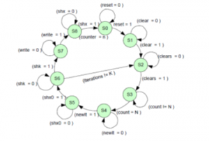
Figure 7: LSP State Diagram

• Countsys S7: Once all K  blocks are processed, memory is initialized in this state to store the results. State transition occurs when Write becomes high.
• Savex S8: In this state, results are updated on the output text file.

All the control signals generated by the state diagram will be reflected in the LSP data path which is as shown in Figure 8.

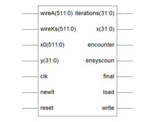
Figure 8: LSP Data Path

4. Results

On Intel Core with 1.2GHz  processor and 3GB  memory, several time experiments are carried out. Obtained results are tabulated to analyze the performance of our proposed architecture. Bellow steps are followed to get the results.

• Select any Image of dimensions more than or equal to 256 X 256 .
• Create a text file in HEX.
• Use text file in Test-bench and reconstruct signal which will be stored in the output text file.
• Read the output text file and display it after processing

Steps 1, 2, and 4 are carried out in MATLAB 2014A. For the third step, the ModelSim PE Student Edition is used. Standard Lena image of dimension 256 x 256  and 512 X 512 with different image formats are used as input to the proposed architecture. Several times process is repeated and only the average value of selected parameters [16] is analyzed.

• MSE: Difference between original and reconstructed signal which is estimated using MSE defined by equation (8).

• Reconstruction time: Time taken by OMP VLSI architecture to generate output file which is measured in second.
• SNR: The amount of noise present in the signal reconstructed using OMP VLSI architecture which is defined by equation (9).

4.1. Analysis of Image Reconstruction Quality

• Standard Lena Image N=256 and 512.
• Measurement Matrix: 128 X 256
• Number of CS measurements = 128X 1.
• FHT transform coder.
• Threshold value (±Tr) = 3

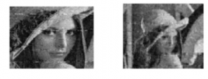
Figure 9: Reconstructed 256 X 256  and 512 X 512  Image

Figure 9 is the reconstructed image using OMP VLSI Architecture indicates that the quality of the image degraded which will be one of the future challenges of OMP VLSI architecture. Simulation results of this work compared with MATLAB implementation [17] and Virtex 5 implantations [18, 19] as shown in Table I. Compared with other simulation work, the proposed design takes less reconstruction time. The reduction in reconstruction time is mainly due to less processing elements as input 3x 3  is fed into the system iteratively. To process 256×256   at a time require more hardware and more time to reconstruct

Table  SEQ Table \* ARABIC 1: Comparison of Proposed Design with Other Similar Work

Platform	[17]		[18]	[19]	Proposed
Tools Used	MATLAB		Xilinx		Xilinx
Target Device	NA		Virtex-5		Virtex-4
Signal Size (N)	256	512	256	256	256
Measurements (m)	128	128	64	64	128
Sparsity Count (K)	64	64	8	8	64
Reconstruction Time	9sec	15sec	17µS	22µS	2.62µS
MSE	550	580	–	–	166.60
SNR (dB)	23	26	–	–	25.91

4.2. Varying Tr  with FHT Domain

Normally large amplitude signals hold most of the important information about the input. Even by neglecting lesser value amplitude signals, information can be extracted. To remove small amplitude signal threshold value from ±2 to ±6 is used in the FHT domain. To minimize the number of measurements larger threshold value should be selected. However, it affects the quality of the reconstructed signal. Therefore trade-off between the quality of the reconstructed signal and reconstruction time will be the parameter for selecting proper threshold value. Experiment analysis shows that for N=256 or 512 , the FHT threshold value should not be more than ±7 . SNR for different threshold is almost the same as shown in table 2.

Table 2: Threshold and SNR Analysis

Image Size	Threshold (±Tr)	SNR (dB)
256 X256	2	25
	4	25
	6	25

4.3. Device Utilities

Table 3 shows the device utilization report using the Xilinx ISE 8.1i version tool. Verilog code implemented on target device namely xc4vlx15-12sf363 (Vertex 4 FPGA). However, our work [1] and [17] are continued in this paper and the main objective of reduction of reconstruction time is achieved. The analysis and optimization of area, power consumption, and other VLSI parameters are considered as future work for this paper.

Table 3: Device Utilization Summary

Logic Utilization	Used	Availability	Utilization
Slices	2116	6144	34%
Slice F/F	2257	12288	18%
4 Input LUTs	3523	12288	28%
Bonded IOBs	212	240	88%
GCLKs	1	32	3%

5. Conclusion and Future Work

This paper presents semi-VLSI architecture which contributes to developing hardware, especially for the Compressive Sensing image. The implemented architecture has equal reconstruction for both 256×256 and 512×512  image i.e 2.62µS  since it is resized to256x256 . This is far better than software implementation and some hardware implementation. For FHT (Foreward Transform)  ±2 to 6  (less than7 ) is to be used as a threshold for proper reconstruction. 25db and 27dB  are the SNR for an image of size 256 x 256   and 512×512  respectively. Mean Square Error (MSE) is 166 which is less as observed in software. Finally, our work concludes that one of the objectives (reconstruction time) is achieved. Analysis and optimization of some objectives like area, power consumption, and other VLSI parameters are considered as future work of this paper

Conflict of Interest

The authors declare no conflict of interest.

1. S. Santosh, V. Siddamal, “A Survey and Theoretical View on Compressive Sensing and Reconstruction”, I.J.Image, Graphics and Signal Processing, 2016, DOI: 10.5815/ijigsp.2016.04.01 MECS Journal
2. D. L. Donoho, “Compressed sensing,” in IEEE Transactions on Information Theory, 52(4), 1289-1306, April 2006.
3. E. J. Candes and M. B. Wakin, “An Introduction To Compressive Sampling,” in IEEE Signal Processing Magazine, 25(2), 21-30, March 2008.
4. Shreyas Joshi, Saroja V. Siddamal “Performance Analysis of Compressive Sensing Reconstruction” IEEE sponsored 2nd International Conference on Electronics and Communication Systems (ICECS 2015), pp-724-729, 26th to 27th February KNU Coimbatore 2015, 978-1-4788-7225-8/15/$31.00 ©2015 IEEE.
5. J. Romberg, “Imaging via Compressive Sampling,” in IEEE Signal Processing Magazine, 25(2), 14-20, March 2008.
6. K. V. Siddamal, Shobha P Bhat, Saroja V. S “A survey on compressive sensing” IEEE sponsored 2nd International Conference on Electronics and Communication Systems (ICECS 2015), pp-639-643, 26th to 27th February KNU Combaiture 2015, 978-1-4788-7225-8/15/$31.00 ©2015 IEEE.
7. R. Baraniuk, M. Davenport, R. DeVore, and M. Wakin. “A simple proof of the restricted isometric property for random matrices”. Const. Approx., 28(3):2538211; 263, 2008.
8. M. Davenport, J. Laska, P. Boufouons, and R. Baraniuk. “A simple proof that random matrices are democratic”. Technical report TREE 0906, Rice Univ., ECE Dept., Nov. 2009.
9. M. Davenport, P. Boufounos, M. Wakin, and R. Baraniuk. “Signal processing with compressive measurements”. IEEE J. Select. Top. Signal Processing, 4(2):4458211; 460, 2010.
10. M. Davenport, J. Laska, P. Boufouons, and R. Baraniuk. “A simple proof that random matrices are democratic”. Technical report TREE 0906, Rice Univ., ECE Dept., Nov. 2009.
11. U. Dias and M. E. Rane, “Comparative analysis of sensing matrices for compressed sensed thermal images,” 2013 International Mutli-Conference on Automation, Computing, Communication, Control and Compressed Sensing (iMac4s), Kottayam, 2013, 265-270.
12. Meenakshi and Sumit Budhiraja, “A survey of Compressive Sensing Based Greedy Pursuit Reconstruction Algorithms”, IJIGSP, 7(10), 1-10, Pub. Date: 2015-9-8
13. J. A. Tropp and A. C. Gilbert, “Signal Recovery From Random Measurements Via Orthogonal Matching Pursuit,” in IEEE Transactions on Information Theory, 53(12), 4655-4666, Dec. 2007.
14. L. Bai, Patrick Maechler, Michel and Hubert Kaeslin, “High Speed Compressed Sensing Reconstruction on FPGA using OMP and AMP”, IEEE 2012.
15. B. Pierre B, Hasan R and Abbes A, “High Level Prototyping and FPGA Implementation of The OMP Algorithm”, in Information Sciences, Signal Processing and their Application Conference, 11th IEEE International Symposium on, 2012.
16. A. Ahmed et al., “Modeling and Simulation of Office Desk Illumination Using ZEMAX,” in 2019 International Conference on Electrical, Communication, and Computer Engineering (ICECCE), 1–6, 2019. DOI: 10.1109/ICECCE47252.2019.8940756
17. S. S. Bujari and S. V. Siddamal, “Image Reconstruction Using Compressive Sensing Technique for Hardware Implementation,” 2018 International Conference on Electrical, Electronics, Communication, Computer, and Optimization Techniques (ICEECCOT), Msyuru, India, 1042-1046, 2018. doi: 10.1109/ICEECCOT43722.2018.9001308.
18. J. L. V. M. Stanislaus and T. Mohsenin, “Low-complexity FPGA implementation of compressive sensing reconstruction,” in Proc. Int. Conf. Comput. Netw. Commun. (ICNC), 671–675, 2013.
19. J. L. V. M. Stanislaus and T. Mohsenin, “High performance compressive sensing reconstruction hardware with QRD process,” in Proc. IEEE Int. Symp. Circuits Syst. (ISCAS), May, 29–32, 2012.

(Click Here)

(Click Here)