1. Introduction

The main objective of a system reliability evaluation is to provide a certain probabilistic information on potential system component failures since a real design project needs to be evaluated in terms of reliability. A system can be defined as a stochastic graph G = (V, E) which contains the vertices set (nodes) and the edges set (links) of the system [1], [2]. The edges and vertices are usually prone to failures. In our system discussions, we claim that the edges go drop by design while the vertices function perfectly. The edge failures should be probabilistic [3]. A system can be described as working if a source vertex communicates with the vertex in the sink. In this case, it called reliability of two-terminal systems [4].

 A cut set is a collection of components whose failure  removes all the connections between the sources and the sinks of the system and thus leads to system failure, but a minimal cut set is a cut set that cannot be delivered in working condition without creating a path from the source to the sink, i.e., each minimal cut set causes system failure [5]. Conversely, the failure rate is not immediate or obvious [6].

In graph theory and computer science, a square matrix representing a finite graph is an adjacency matrix. The matrix elements indicate whether or not the vertical pairs are adjacent to the graph. The adjacent matrix for a finite simple graph is a (0,1) matrix with zeros at its diagonal [7]. The adjacent matrix is symmetrical if the graph is undirected (i.e. all its edges are bi-directional). The adjacent graph matrix should be separated from its incidence matrix [8]. We construct a set of minimal path set based on the matrix properties of the graph and then use the algebraic properties and multiplication to find the system’s minimal cut set.  Song and Kang [9], [10]  presented a matrix-based system reliability approach which can be tested with simple matrix calculations for evaluating the reliability of complex system stats.  Hassan and Mutar [11]  have recently researched the architecture of electrical device reliability models (geometry point of view) used within spacecraft, which is considered a spacecraft’s high-pressure oxygen supply system (HPOSS) [12]. With exception of current system reliability approaches, the complexity depends heavily on the details. The complexity of the formulas is not affected as the efficiency of the method is calculated with simple matrix calculations.

A connection matrix is a matrix with rows as minimal path sets and columns representing system components, then compared it to the system truth matrix. Based on some algebraic properties, this relation results in minimal cutting sets of the  system. So the Matrix-based minimal cut structure of the system can be accomplished through algebraic manipulation of the transpose of a incidence matrix with the truth matrix . From that, we form a matrix in which the rows represent the minimal cut, and columns represent the components of the system then, we find the reliability of the system or obtain information about the system failure. Generally, this method is used to find the reliability of systems by using the Mathematica software.

This paper presents a minimal cut method based on matrix and applies it to a simple system and engineering structures (look- ing at as networks), as seen in Figure 1. The units may be linked as a complex configuration. In a spacecraft, that reflects a HPOSS, i.e. the HPOSS in the cabin by the array of controls and valves from a high-pressure oxygen tank. This system consists of several components connected in a complex form for quantifying. The Matrix-based minimal cut analysis uses the representation of the incidence matrix whose elements indicate whether vertex–edge pairs are important in evaluating the minimal path sets of the systems. Then the  matrix of minimal cut formulation of a system can be obtained depending on the minimal path sets of the  systems. Generally, for solving complex models, we give an algorithm for calculating all minimal cuts, we use the Mathematica program to implement. We also gives powerful ideas to understand the MTTF of complex systems [13].

2. Models of network reliability

A reliability block diagram of a system is a graph whose edges are the system components, while there exists a pair of nodes called terminal nodes, in the backup power supply diagram. This describes the functional relationship between the components, and indicates if there exists a path between the terminal nodes which contains only edges with functional components (making, consequently, the entire system functional; in the contrary case, this is non-functional). It shows the functional relationship between the components, and indicates there is a path between the terminal nodes that contains only edges with functional parts. Otherwise it is not functional. The graphical model represents the reliability structure of the system like series , parallel and complex structures.

The system S consists of n components  which can only work or fail in one of two states. Then we can define the boolean (binary) indicator variables for each component or S system for these states. The system design and connection paths reflect the reliability structure of the system which might or might not be the system’s functional block diagram. As a practical illustration of engineering systems, modules can then be attached to a complicated configuration as illustrated in Figure 1. is a spacecraft’s high-pressure oxygen supply system (HPOSS) [11] [12].

Figure 1:  Reliability block diagram of system S.

As an illustration, we will study a simple model is a basic reliability block diagram with 3 subsystems as Figure 2, then we formulate a general Algorithm for complex models.

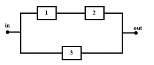
Figure 2:  Reliability block diagram of system S.

3. Matrix-based minimal path deduction

The graph G = (V, E) represents the components’ logical relations inside a piece of equipment. It is not necessarily the graphical representation of the system, but the system’s functional components. In the graph theory, the minimal path is the problem of selecting a path from which no component can be removed without disconnecting the connections between the scour and sink node in a graph such that the sum of its constituent edges is minimized.

Consider a system that has different states with its  component, . The connection matrix (CN) is constructed in order to create the minimal paths by adding a (n × n) adjacent matrix of a simple graph with the identity matrix (unit matrix) in size n, to obtain 1’s in the main diagonal, that is

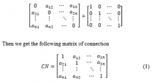
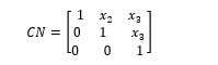
where  is the set of vertices, and    is the edge between vertex i and vertex j, if there is a connection between vertex i and vertex j then  , otherwise   .For example , in Figure 1, the simple model has the following connection matrix

Therefore, we finding the minimal path between a two-terminal system as a special case of the paths problem, the minimal path vector for a system can be constructed by removes vertices which are either source or sink in the (CN) matrix, one at a time, until only the source vertex and sink vertex are present in the matrix [13]. When a vertex is deleted, the connection matrix inputs are modified using the following equation for the remaining vertices:

if vertex l is removed, where  and  for  . Otherwise   iff .

The system shown in Figure 2 can be formulated as graph with directed edge (component) ?? of simple model is a basic RBD with 3 subsystems for ? ??? ?= 1,2,3. So the all minimal paths of the system are .

Generally, for finding all minimal paths of series, parallel and complex system. A minimal path deduction algorithm  to calculate all the minimal paths [14]. Based on the communication matrix and equation (1) by using the Mathematica software.

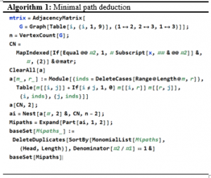
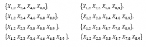
Applying the algorithm (1) to the complex model in Figure 1, all the minimal path sets can be obtained

The use of this approach is good practice by marking the source vertex as the first vertex and the sink vertex as the last vertex. Each intermediate node is deleted one by one until a 2×2 matrix is left with  represent summation of all minimal paths. Therefore, removing node  implies removing row  and column  from the original connection matrix where  for a network with perfect n nodes [2].

4. Matrix-based minimal cut deduction

This method is based on minimal path mainly. The incidence matrix of minimal paths can be obtained from all minimal paths by use of a set of all minimal paths [3]. Assume that n minimal paths are defined by . These paths will create a matrix while the paths represent the rows and the components represent the columns of the matrix. we determine the incidence matrix (IM) of all the minimal paths, of the form:

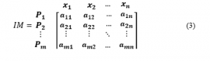
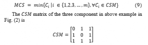
where  with  and  iff , otherwise  . Appling to the system illustrated in Figuer 2, we obtain incidence matrix as follows.

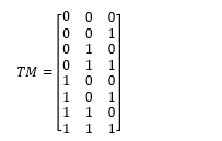
Based on the algebraic properties, we can form the truth matrix (TM) depending on the listing of a limited number of system s ates, which is the most common approach. The true matrix of the graph is an n-dimensional vector consisting of 1s and 0s in raws and the components represent the columns of the matrix. If the  of a state is 1, component i shall be in that state; otherwise it shall be down, illustrates the system model in Figure 2 its sample space divided into  . The TM matrix of the three component sates is

      Then, we perform the multiplication process between the transpose of a incidence matrix (IM) and the truth matrix (TM)  such that incidence matrix is  n × m matrix  and the truth matrix is p × m matrix , then A is an p × n matrix with entries, so the comparison matrix is ​​formed as in the equation

   

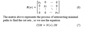
  The process of this multiplication produces a new matrix that represents a fracture that helps to find parts and malfunctions in the system and the components that stop that we use the least property of Boolean algebra between the elements of the matrix rows according to the formula:

      So for above example  Whereas, this object represents the diameter elements in a matrix that  create with, then we Then we make  and remove the zero rows of the previous result. This is a job for logical indexing. Then we take

The  matrix include all cuts in rows and the components are arranged according to the columns in sequence , then the conditions of component failures are given by a single matrix.

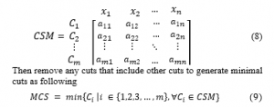
Then remove any cuts that include other cuts to generate minimal cuts as following

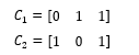
For the edge ??, the minimal cut is .

Generally, for finding all minimal cuts of series, parallel and complex system. A minimal cut deduction algorithm  to calculate all the minimal cuts [14]. Based on the CSM matrix and equation (9) by using the Mathematica software.

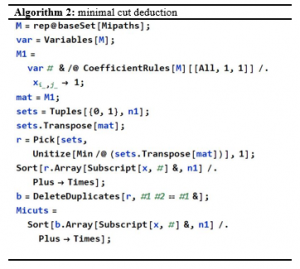
Applying the algorithm to the complex model in Figure 1, all minimal cuts can be obtained

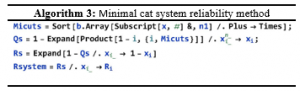
5. Minimal cat system reliability method

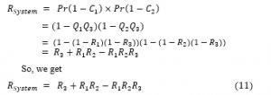
This method determines the reliability of a systems by using the minimal cut set and the inclusion-exclusion rule [15]. A cut Set is a set of components that fail to interrupt all the connections between source and sink, which causes device failure [16]. Then the system reliability can be written as

where  represent all the minimal cuts, and where  . Therefore, the probability of system failure is determined by a simple vector calculation

For example , in Figure 2, the system model has the following minimal cut vectors

So the minimal cut are  . These Reliability System  can be generated easily by using the Mathematica software. Using equation (10) subsequently, the Reliability System  is obtained as

In general, the Reliability System for the union of minimal cuts is obtained using Mathematica processes

      The minimal cut method based on the matrix has Firstly, as a result of calculating the connection matrix independently from a system definition, the reliability of a system event is calculated, the complexity of system reliability evaluations is not related to the concept of system states. Secondly, the matrix-based method helps one to understand easily and solve the failure rate of the system. Third, if component failure probabilities or statistical dependency are incomplete, the matrix-based method helps one to achieve the shortest possible limit for all general system states. Fourth, recent developments in matrix-based computer languages and software, including Mathematica software, have made it easier and more efficient to implement matrix calculations. Finally, in this paper, the examples deal with two-state systems. The proposed approach is applicable to general multi-state component systems.

6. The Mean Time to Failure (MTTF)

The transformations we use are called linearizing transformations, which researchers have used in the past to evaluate the values of constants to best match a collection of data. The exponential function is of the form , and the ln-transformation of R(t) matches it with , mapping an exponential to a linear expression [17]. In particular, this approach refers to circumstances where the rate of the quantity change is directly commensurate with the radioactive decay (see [18], p.483] for further details). The exponential function also represents a curve whose form mainly depends on the exponent ‘s constant.

• If a > 0, then R(t) increases as t increases,
• If a < 0, then R(t) decreases as t increases.

Because of the interpretation of the Mean Time to Failure, we obtain

where  and : The function (15) is decreasing and satisfies the Reliability conditions. Let us also consider the polynomial of reliability (11). We assume that exponential functions correspond to , where  and , for . Then we obtain

The above relationship through which it is possible to deduce the time for the failure of the system and then relay the components to give the longest time as a system.

7. The failure rate of the system reliability

In order to evaluate the system failure rates for the reliability system (11) used as a simple example with constant failure rate components. Consider the equation (12) of one component;

the reliability of the component selected is given

The failure rate is defined as the relationship between the density of probability and the reliability function

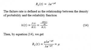
The failure rate of the system for the failure rate of components in the complex system as constants is therefore time-related [19]. We find that if the component failure rate is constant, the system failure rate is also constant. In other words, the system’s failure rate is always equal to the stable state failure rate [20].This is thus an correct representation of the state of polynomial multivariate reliability based on the values of the constants .

A practical example of engineering systems has been used with the proposed algorithm, components can be connected in a complex system, as shown in Figure 1. Including 9 nodes and 9 edges. The patterns representing system states and component problems can be defined effectively using matrix-based programming languages and applications. In addition, we obtain the failure rate equation, which results in an incremental failure of one variable being reduce by improving the pairing component, and which, obviously, provides a mathematical basis for the failure rate. This result demonstrates that our approach increases accuracy without increasing the assessment time.

8. Conclusions

This paper clearly defines a new method of deducing minimal cuts according to minimal path sets of complex systems, using the minimal cuts approach in a simplified form. The Matrix-based minimal cat approach can calculate the Reliability of complex system states by simply calculating matrix. Using matrix-based programming languages and applications, the matrices representing the system states and the component problems can be effectively defined. The components (the system) also proven to be exponentially time dependent; furthermore, we achieve a failure rate equation indicating that a gradual failure of a component can be balanced by the improvement of the pairing component, and naturally gives a mathematical foundation for the failure rate.  When the states of component failure are dependent largely. In some instances, we find a state failure rate and display certain components to be the efficient elements responsible for the device failure.

1. Y.H. Kim, K.E. Case, P.M. Ghare, “A method for computing complex system reliability,” IEEE Transactions on Reliability, 21(4), 215–219, 1972, doi:10.1109/TR.1972.5215997.
2. W. Kuo, M.J. Zuo, Optimal reliability modeling: principles and applications, John Wiley & Sons, 2003.
3. J.-L. Marichal, “Structure functions and minimal path sets,” IEEE Transactions on Reliability, 65(2), 763–768, 2016, doi:10.1109/TR. 2015.2513017.
4. S. Kharbash, W. Wang, “Computing two-terminal reliability in mobile ad hoc networks,” in 2007 IEEE wireless communications and networking conference, IEEE: 2831–2836, 2007, doi:10.1109/WCNC. 2007.525.
5. R.N. Allan, Reliability evaluation of power systems, Springer Science & Business Media, 2013.
6. S.M. Alghamdi, D.F. Percy, “Reliability equivalence factors for a series–parallel system of components with exponentiated Weibull lifetimes,” IMA Journal of Management Mathematics, 28(3), 339–358, 2017, doi:10.1093/imaman/dpv001.
7. G.T. Gilbert, “Positive definite matrices and Sylvester’s criterion,” The American Mathematical Monthly, 98(1), 44–46, 1991, doi:10.1080/000 29890.1991.11995702.
8. M.B. Javanbarg, C. Scawthorn, J. Kiyono, Y. Ono, Minimal path sets seismic reliability evaluation of lifeline networks with link and node failures, 1–12, 2009, doi:10.1061/41050%28357%29105.
9. W.-H. Kang, J. Song, P. Gardoni, “Matrix-based system reliability method and applications to bridge networks,” Reliability Engineering & System Safety, 93(11), 1584–1593, 2008, doi:10.1016/j.ress.2008. 02.011.
10. W.-H. Kang, Y.-J. Lee, J. Song, B. Gencturk, “Further development of matrix-based system reliability method and applications to structural systems,” Structure and Infrastructure Engineering, 8(5), 441–457, 2012, doi:10.1080/15732479.2010.539060.
11. Z.A.H. Hassan, E.K. Muter, “Geometry of reliability models of electrical system used inside spacecraft,” in 2017 Second Al-Sadiq International Conference on Multidisciplinary in IT and Communication Science and Applications (AIC-MITCSA), IEEE: 301–306, 2017, doi:10.1109/AIC-MITCSA.2017.8722980.
12. K.K. Aggarwal, Reliability engineering, Springer Science & Business Media, 2012.
13. Y. Kobayashi, M. Hayashi, “A new approximation method to evaluate system reliability,” in 2017 IEEE International Symposium on Local and Metropolitan Area Networks (LANMAN), IEEE: 1–2, 2017, doi:10. 1109/LANMAN.2017.7972141.
14. S.S. Skiena, The algorithm design manual: Text, Springer Science & Business Media, 1998.
15. K. Dohmen, “Inclusion-exclusion and network reliability,” The Electronic Journal of Combinatorics, R36–R36, 1998, doi:10.37236/ 1374.
16. J.E. Biegel, “Determination of tie sets and cut sets for a system without feedback,” IEEE Transactions on Reliability, 26(1), 39–42, 1977, doi:10.1109/TR.1977.5215071.
17. Z.A.H. Hassan, C. Udriște, “Equivalent reliability polynomials modeling EAS and their geometries,” Annals of West University of Timisoara-Mathematics and Computer Science, 53(1), 177–195, 2015, doi:10.1515/awutm-2015-0010.
18. T. Pyzdek, P.A. Keller, Quality engineering handbook, CRC Press, 2003.
19. L. Xu, Y. Chen, F. Briand, F. Zhou, M. Givanni, “Reliability measurement for multistate manufacturing systems with failure interaction,” Procedia CIRP, 63, 242–247, 2017, doi:10.1016/j.procir. 2017.03.124.
20. H. Pham, “Commentary: Steady-state series-system availability,” IEEE Transactions on Reliability, 52(2), 146–147, 2003, doi:10.1109/TR. 2003.811164.

(Click Here)

(Click Here)