1. Introduction

Cardiovascular diseases are main reseaon of death in the United States, accounting for a large proportion of deaths around the world [1]. According to the World Health Organization, about 15 million people die annually from cardiovascular disease in the world and this includes 30 percent of all deaths [2].

1.1. Familiarity and Perceptions of heart disease

Heart disease includes conditions such as coronary heart disease, ischemic heart disease, heart attack, cardiac arrhythmia, cerebrovascular disease and other conditions [3]. Cardiac ischemia, heart injury and heart attack are three consecutive stages in which coronary arteries proceed from congestion to full blockage. Ischemia means limited blood supply. In cardiac ischemia, the muscle suffers from a lack of oxygen due to the narrowing of the arteries that supplying blood to the heart and this leads to the reduction in blood flow to the heart. Therefore, there is a mismatch between the blood supply and the blood demand in the heart, and this imbalance can lead to the heart tissue death [4]. Heart injury is a condition in which the blood supply to the heart continues to decline beyond ischemia and tissue damage begins. This condition still can be avoided as no sign of a heart attack has observed [4]. A heart attack or infarction is a condition in which the blood supply to the heart stops and the death of part of the tissue occurs, which is mainly causes by a blockage of the coronary artery following a rupture in the plaque artery wall [5]. An adult’s healthy heart during resting usually beats 60 to 100 times a minute. The heart rate below 60 beats per minute at rest is called bradycardia, and a heart rate more than 100 beats per minute at rest is called tachycardia. Sinus bradycardia is a type of slow beating that occurs when the problem starts in the sinoatrial node (SA). The SA node of the heart is the natural pacemaker in the heart. If the electrical impulses in the sinus node are not generated properly, sinus bradycardia will occur. In sinus tachycardia, the SA node regularly produces constant beats ranging 160 to 180 beats per minute [6].

Myocardial fibrosis, myocardial infarction, myocardial inflammation, pulmonary embolism, and coronary artery diseases cause the damage to the bundle branch blocks of the heart. Bundle branch blocks are a group of blocks in which the ventricles cannot be depolarized at the same time due to conduction disturbances in the conductive fibers inside the ventricles, and as a result the QRS complex changes in terms of time duration or shape. In the right bundle branch block, there is a conductive disturbance in the right bundle branch of the His, and first the left ventricle is depolarized in normal path, then the right ventricle is depolarized with a delay. Also, in the left bundle branch block, the dysfunction of the left bundle branch of His causes normal depolarization of the right ventricle and delayed depolarization of the left ventricle [7,8].

1.2. Applying pattern recognition methods in identifying heart diseases

Nowadays, in many cases, machines have replaced humans, and most of the physical work that used to be done by humans is now being performed by machines. Although the power of computers in storing, retrieving information and etc. is undeniable, still there are some cases that humans have to do alone. But in general, machine-related cases involve systems in which the human brain is unable to mathematically understand these connections due to the complex connections between components. Over time, the human brain can partially identify the habits of the system by observing the sequence of behaviors of the system and sometimes testing the results obtained by manipulating one of the components of the system. This learning process leads to experience by observing various examples of the system. In such systems, the brain is unable to analyze the system internally and only estimates the system’s internal performance and predicts its reactions based on external behaviors. How to manage large amounts of information and use it effectively to improve decision-making is one of the most challenging issues in the modern era. One of the most important research issues in computer science is the implementation of a model similar to the internal system of the human brain for the analysis of various systems based on experience. In this regard, neural networks are one of the most dynamic areas of research in the current era.

The different information received from different channels, along with the general information of individuals, creates a lot of numbers in order to diagnose different heart diseases. This large amount of information makes it difficult to establish pattern recognition structures on one hand, as well as increases detection time on the other hand. In order to use microcontroller systems independent from computers, it is vital to reduce the amount of information received from the person under the study. Also, due to the much lower speed of microcontroller systems compared to computers, this volume reduction will be very significant in the speed of program execution.

Microcontrollers are microprocessors that, in addition to CPU, at least include input and output systems, memory, and memory-connected circuits inside the main chip, and they do not require external intermediary circuits to connect to additional systems. Of course, all microcontrollers are not similar, and some microcontrollers in addition to considerable features include digital to analog and analog to digital converters, or even more facilities. Using advanced architecture and optimal commands, microcontrollers reduce the amount of code generated and increase the speed of program execution. Therefore, a simple microcontroller is used for classification with high accuracy and speed [9].

The present study focuses on the role of each of the features in  diagnosis of heart disease, so, we should first mention sampling method and calculating each of the features.

2. Sampling Method

2.1. Obtaining information about heart function

Cardiac signals are received by metal electrodes attached to the limbs and chest and amplify and record by ECG. As shown in figure 1, there are 12 leads in a complete electrocardiography, which include 6 limb leads and 6 chest leads or precordial. Limb leads has two types: standard bipolar leads and amplified unipolar leads. Bipolar leads consist of three leads and are called lead I and II and III or L1 and L2 and L3, and indicate the potential difference between the two points of the body [10].

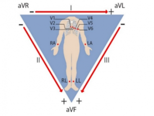
Figure 1: Limb and chest leads [11]

An electrocardiogram (ECG) or ECG is a written record of the potentials generated by the heart that includes specified areas shown in figure 2.

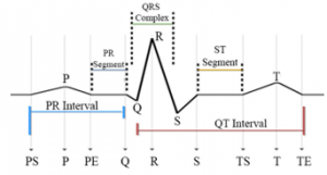
Figure 2: Different areas of an electrocardiogram [12]

In this study, the features of cardiac arrhythmia database were examined. As illustrated in table1, total number of features are 279.

Table 1: All features table

Status	Number of features	Features Name
1	12,14	Vector angles in degrees on front plane of P,J
1	19,31,43,55,67,79, 115,127,139,151	Average width of R’ wave of channel DI,DII,DIII, aVR, aVL, aVF,V3,V4,V5, V6
1	20,32,44,56,68,80,92, 104,116,128,140,152	Average width of S’ wave of all channels[1]
1	22,34,46,58,70,82,94, 106,118,130,142,154	Existence of ragged R wave of all channels
1	23,35,47,59,71,83,95, 107,119,131,143,155	Existence of diphasic derivation of R wave of all channels
1	24,36,48,60,72,84,96, 108,120,132,144,156	Existence of ragged P wave of all channels
1	25,37,49,61,73,85,97, 109,121,133,145, 157	Existence of diphasic derivation of P wave of all channels
1	26,38,50,62,74,86,98, 110,122,134,146,158	Existence of ragged T wave of all channels
1	27,39,51,63,75,87,99, 111,123,135,147,159	Existence of diphasic derivation of T wave of all channels
1	54	Average width of S wave of channel aVR
1	100,112, 124	Average width of Q wave of channel V2,V3,V4
1	165,175,185,195,205, 215,225,235,245,255, 265,275	Amplitudes of S’ wave Of all channels
1	160,162,163	Amplitudes of JJ,R,S waves Of channel DI
1	164,174,194,204,214, 234,244,254, 264,274	Amplitudes of R’ wave Of channel DI,DII,aVR,Avl, aVF, V2,V3,V4,V5,V6
1	161,231,241,251	Amplitudes of Q wave Of channel DI,V2,V3,V4
2	10	Vector angles in degrees on front plane of QRS
2	16	Average width of Q wave of channel DI
2	41,101,113	Average width of R wave of channel  DIII,V2, V3
2	66, 78	Average width of S wave of channel aVL, aVF,
2	105	Number of intrinsic deflections of channel V2
2	173,176	Amplitudes of S,P waves Of channel DII
2	252,253	Amplitudes of R,S waves Of channel V4
2	261,262,263	Amplitudes of Q,R,S waves Of channel V5
2	272	Amplitudes of R wave Of channel V6
2	187	Amplitudes of T wave Of channel DIII
2	178,208,228	QRSA of channel DII, aVL,V1
2	199,219,269	QRSTA of channel aVR, aVF,V5
2	190,210,220,230,260, 270	Amplitudes of JJ wave Of channel aVR,aVF,V1,V2,V5, V6,
2	192,193	Amplitudes of R,S waves Of channel aVR
2	201	Amplitudes of Q wave Of channel aVL
2	242,243,247	Amplitudes of R,S,T waves Of channel V3
3	5	QRS duration
3	6,7,8,9	P-R,Q-T,T,P intervals
3	11,13	Vector angles in degrees on front plane of T, QRST
3	28,40,52,64,76,88, 136,148	Average width of Q wave of channel DII, DIII, aVR,aVL, aVF,V1,V5,V6
3	17,29,53,65,77, 89, 125,137,149	Average width of R wave of channel DI,DII,aVR, aVL, aVF, V1,V4,V5,V6
3	18,30,42,90,102, 114, 126,138,150	Average width of S wave of channel DI,DII, DIII,V1, V2, V3, V4,V5,V6
3	21,33,45,57,69, 81,93, 117,129, 141,153	Number of intrinsic deflections of channel DI,DII, DIII,aVR,aVL, aVF, V1, V3,V4,V5,V6
3	91,103	Average width of R’ wave of channel V1,V2
3	166,186,196,206,216, 226,236,246,256,266, 276	Amplitudes of P wave Of channel DI, DIII, aVR, aVL, aVF,V1,V2, V3,V4, V5,V6
3	167,177,197,207,217, 227,237,257,267,277	Amplitudes of T wave Of channel DI,DII,aVR,aVL, aVF,V1,V2,V4, V5,V6
3	171,181,191,211,221, 271	Amplitudes of Q wave Of channel DII,DIII,aVR,aVF, V1,V6
3	170,180,200,240,250	Amplitudes of JJ wave Of channel DII,DIII,aVL,V3,V4
3	172,182,202,212,222, 232	Amplitudes of R wave Of channel DII,DIII,aVL,aVF, V1,V2
3	183,203,213,223,233, 273	Amplitudes of S wave Of channel DIII,aVL,aVF,V1, V2, V6
3	184,224	Amplitudes of R’ wave Of channel DIII,V1
3	168,188,198,218, 238,248,258,268,278	QRSA of channel DI, DIII, aVR,aVF,V2,V3,V4,V5,V6
3	169,179,189,209,229, 239,249,259,279	QRSTA of channel DI,DII, DIII,aVL,V1,V2, V3,V4,V6
4	1	Age
4	2	Sex
4	3	Height
5	4	Weight
5	15	Heart rate

The features include general specifications and ECG signals received from patients. In ECG signals received from the patients, the channels are DI, DII, DIII, aVR, aVL, aVF, V1, V2, V3, V4, V5 and V6, respectively. Features of status 1 have zero or close to zero values, features of status 2 have a negative effect on classification, and features of status 3 are combined features. The main features of 1,2,3, which are defined as status no. 4, and the combined features of 5,14,17 are removed due to their low effect on classification accuracy. Also, features 4 and 15 remained constant from the beginning to the end of the process, which can be observed in table 1 as status number 5.

3. Neural Networks

A neural network is one of the most popular classifiers in various researches, especially the classifiers related to heart disease, and etc [13-16].

Among different neural networks, the possibility of implementing perceptron neural networks in microcontrollers is more. The ability to link Arduino microcontrollers to the Simulink environment in Matlab, has made it possible to transfer Perceptron neural networks into Arduino microcontrollers regarding to  memory-related items and etc.

3.1. Perceptron Neural Network

One type of neural network is the perceptron neural network which is divided into Single- Layer Perceptron (SLP) and Multi- Layer Perceptron (MLP). Perceptron neural networks are classified as feed forward neural networks. A single layer perceptron can only categorize separate linear problems, and for more complex problems we need to use more layers. Multi-layer feed forward networks consists of one or more middle layers. The multilayer perceptron is a completely interconnected network because each neuron in one layer is connected to all the neurons in the next layer. If some of these connections do not exist, the network is an incomplete connected network [17].

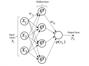
Figure 3: An example of Multi-layer perceptron neural network [18]

The input-output equations of kth neuron are as follows:

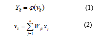
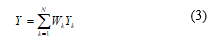
where  are input signals.  is the output of the sum.  are the weights of neurons. The final output of the MLP network with a hidden layer is equal to:

The active function used in the hidden layer is usually nonlinear. And the transform function in the output layer can be linear or nonlinear.

The Perceptron algorithm is a repetitive algorithm, in which the weight and bias vectors are first quantified, and then at each step, the algorithm changes the weight and bias values ​​according to the points that are not accurately categorized to categorize these points correctly. If the given points are not linearly separable, the perceptron algorithm will not end, but if the linear points are separable, the algorithm will end in finite number of steps.

4. Data Analysis

Using all the features, we use a classification to remove and combine low-value features using different methods to improve the accuracy and speed of the neural network.

4.1. Classification with all features

Before analyzing the features, firstly a classification has made in order to evaluate the whole system considering all features. A single layer network is designed as shown in Figure 4.

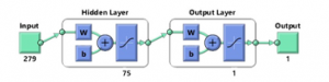
Figure 4: Neural network with four classes considering all features (279 features)

By changing all possible parameters in a Perceptron neural network, including the number of hidden layers, the number of neurons in each layer, and the transform functions of each neuron, the best possible accuracy for the neural network and with the accuracy of 92.324% obtained as shown in figure 5.

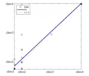
Figure 5: Neural network regression with all 279 features with 92.324% accuracy

The points outside the dash- line indicate an error in classification with the neural network as shown in figure 4.

4.2. Removing features with values ​​close to zero

By studying all the samples, some of the features that had zero value (25 features) or very close to zero (104 features) in all samples were removed from the features. The number of features was reduced from 279 to 150, and the number of features removed at this stage is 129. These features are shown in table 1 as status number 1. By removing the features close to zero, with 150 remaining features, the perceptron neural network has re-formed with a hidden layer as shown in figure 4 with 100 neurons in that layer, and with the optimization of its various parameters, as shown in figure 6 the classification accuracy has increased from 92.324% to 94.579%. The accuracy obtained at this stage indicates the accuracy of our performance in removing the features close to zero.

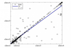
Figure 6: Neural network regression with 150 features after removing features with values ​​close to zero with an accuracy of 94.579%

4.3. Studying the effect of each feature on neural network error rate

To calculate the effect of each feature on the error of neural network, we consider a figure similar to figure 7 as a neural network with one output, which the transform function of each neuron is  and the number of neurons in the middle layer is .

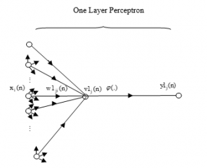
Figure 7: Perceptron neural network output layer with partial specifications

If the optimal output of the network is d and its actual output is y, the network error is defined as follows:

The total error of a neural network is defined as the sum of the output errors and based on considering an output in the network of figure 7, we have:

On the other hand, according to the weights of the final layer, the input of the last layer neuron is defined as follows

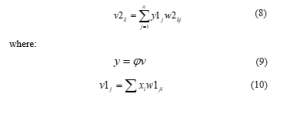
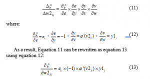
To calculate the effect of the weights of the layer shown in figure 7 at the total output of the network , can be written:

To calculate the effect of pre-final layer weights, consider a figure similar to figure 8.

Considering Equation 13, we can define the effect of the weights of pre-final layer on the total error as follows:

Now it is enough to calculate the effect of each of the features on total error using the following Equation:

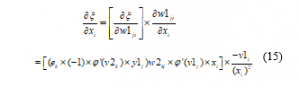
As all the weights of the last layer affect the total error through each of the features, thus:

At this stage, 6 different neural networks of Perceptron have designed with different parameters and by applying and not applying any of the features in all designed networks, the effect of each feature on the error ratio of classification of the networks has been calculated.

Studying figure 10, 35 features that had caused adverse effects in classification of more than 4 neural networks and were marked red, have identified and removed. These features are shown in Table 1 as status number 2. By removing the specified features, the number of features has reduced from 150 to 115, and again a Perceptron neural network with a hidden layer as shown in figure 4 with 105 neurons in that layer has optimized for classification of different features.

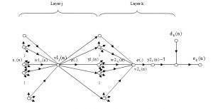
 Figure 8: A more detailed view of the output and hidden layers of the Perceptron neural network

The classification accuracy for this neural network, as shown in figure 9, is 97.155%, which has improved compared to the neural network of previous stage with accuracy of 94.579%.

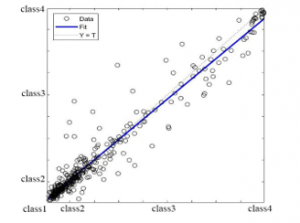
Figure 9: Neural network regression designed with 115 remained features from stages 4-2 and 4-3 with 97.155% accuracy

4.4. Combining features

After removing features with values ​​close to zero as well as features with negative effects on the accuracy of neural network’s classification, according to Fisher’s discriminant ratio (FDR) and applying optimization on it the remaining 115 features are combined in multiple groups and present the formation of features with suitable performance and more discriminant power among the classes.

To describe the performance of FDR, at first in a two-classes case, it is assumed that the data have Gaussian or quasi-Gaussian distribution. As shown in figure 10, if the average difference between the features of the two classes has increased and their variance have gotten smaller, the discrimination of these two classes will be improved.

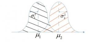
Figure 10: Diagram of detecting the degree of discrimination of two classes [19]

As mentioned, the FDR is defined as follows:

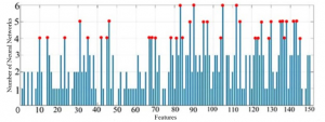
Figure 11: The number of negative effects of each feature on different neural networks tested

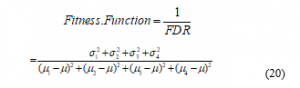
If the difference between means increases and the variances decreases, the FDR increases. Therefore, increasing FDR means increasing class separation and thus increases the accuracy of classification. Now, if Equation (17) is generalized to a 4 –classes case, we have:

To achieve optimization possibility (maximizing) the FDR value, a parametric weight is considered for each of the features considered for the combination. For example, to combine n features, weights with the form are applied to the given features. Then, using genetic optimization algorithm, the values ​​of these coefficients are determined in such a way that the given FDR is maximized.

The genetic algorithm method is based on minimizing the objective function, but since the goal is to maximize FDR, the fitness function of the genetic algorithm is defined as follows:

For example, the features presented in table 2 are combined with the coefficients shown, and after maximizing the FDR with the genetic algorithm, has turned into an optimized feature.

Table 2: Features considered for the combination stated for example

Feature	Coefficient
Amplitude of JJ wave of channel DII	a1
Amplitude  of JJ wave Of channel DIII	a2
Amplitude  of JJ wave Of channel AVL	a3
Amplitude  of JJ wave Of channel V3	a4
Amplitude  of JJ wave Of channel V4	a5

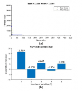
Figure 12: (a) Optimized fitness function for different generations of genetic algorithms (b) Optimized coefficient charts

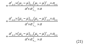
How to apply the coefficients in Equation (20) is considered as follows:

After optimization, the optimal value of the fitness function and the values ​​of each of the coefficients are shown in figure 12.

As shown in Figure 12.b, after optimizing ,  ,  ,  ,  and instead of the features listed in Table 2, the following single features is replaced:

New feature combined

= a₁*Amplitude of JJ wave of channel DII

+ a₂* Amplitude of JJ wave of channel DIII

+ a₃* Amplitude of JJ wave of channel aVL

+ a₄* Amplitude of JJ wave of channel V3

+ a₅* Amplitude of JJ wave of channel V4

Similarly, most other available features are combined in the same way as shown in table 3.

With the processing so far, the number of features has been reduced from 279 to 20. To evaluate the accuracy of the performed processes, again, an optimized Perceptron neural network has designed with a hidden layer as shown in figure 4 with 20 neurons in that layer, and with the remaining 20 features, the accuracy of the classification is 100%, which can be seen in figure 13 of the neural network regression line and in comparison with the regression line of figure 9 with accuracy of 97.155%, the optimal performance of the neural network is observed.

Table 3: Classification of features combined with the values ​​of the coefficients obtained from the genetic algorithm

The number of feature created from the combination	Combined members	Coefficient values
1	28 40 52 64 76 88 136 148	16.495 5.046 5.027 -5.429 -10.297 4.963 19.642 -19.996
2	17 29 53 65 77 89 125 137 149	16.519 5.023 4.99 -5.414 -10.298 4.944 19.612 -19.993 1.465
3	18 30 42 90 102 114 126 138 150	19.56 11.841 4.154 -6.005 -14.663 5.76 -9.814 5.654 9.157
4	91 103	11.651 7.387
5	21 33 45 57 69 81 93 117 129 141 153	19.717 12.501 11.184 -13.653 6.319 0.819 0.489 -15.581 -2.518 -4.174 -0.581
6	170 180 200 240 250	19.472 -9.577 7.04 -1.597 6.314
7	171 181 191 211 221 271	19.736 -9.717 7.124 -1.611 6.386 16.633
8	172 182 202 212 222 232	2.202 2.933 11.031 0.256 -19.972 2.034
The number of features created from the combination	Combined members	Coefficient values
9	183 203 213 223 233 273	-2.148 -2.801 -10.351 -0.125 18.791 -1.917
10	184 224	-10.374 16.532
11	166 186 196 206 216 226 236 246 256 266 276	-1.103 -3.814 2.629 0.742 -0.72 -6.062 3.689 -2.338 -9.028 -5.158 19.995
12	167 177 197 207 217 227 237 257 267 277	19.997 -2.209 1.261 -5.925 6.124 1.926 -3.214 3.267 1.572 5.651
13	168 188 198 218 238 248 258 268 278	-2.421 14.644 -0.308 -13.025 9.193 -3.083 6.634 -19.895 15.906
14	169 179 189 209 229 239 249 259 279	-2.421 14.644 -0.308 -13.025 9.193 -3.083 6.634 -19.895 15.906
15	11 13	6.067 5.972
16	5 6 7 8 9	-18.087 -17.804 14.276 -9.757 -8.759
17	5 6	-14.284 -5.04

Figure 13: Neural network regression with 20 remaining features after combining features with 100% accuracy

4.5. Selection of final features with Principle Component Analysis (PCA) algorithm

Usually the last step in optimizing and selecting features, is the stage of eliminating no-effect or low-effect features. As the combined features lead to FDR optimization and as a result the classification has reached the most accurate state, it is possible to keep the accuracy of the classification  at 100% by eliminating the features that do not have a good effect on classification. To better separation of classes, sometimes you need to make changes to the features. Previously, the application of coefficients to features in order to increase the FDR classification value was investigated. A more general method is now being considered that, in addition to applying coefficients to the feature, also has the ability to make more fundamental changes

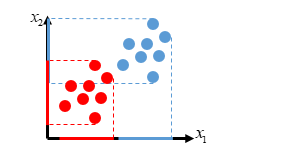
Figure 14: Two-class data arrangement with two features

As shown in figure 14, the two classes with their data are characterized. For these two classes, two features x1 and x2 are considered. Given the degree of separation of class ranges on the axis of each feature, we will notice better discrimination of the x1 feature than the x2.

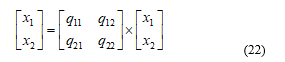
But if it is possible to make changes to the features of the same problem so that the features have a rotational value of the appropriate amount and shape, then the rotated feature of x1 will have more discrimination ability. How to make these changes to the features so that the maximum discrimination is achieved and also the selection of the top features from the classification point of view, is done using a method called PCA. Mathematically, to make any changes, an interface matrix should be used to make any changes. For example, we will have two features:

As shown in figure 15 by adjusting the q values correctly, a suitable change can be made to the features so that the data scatter is properly adjusted and thus the classes’ discrimination is simplified.

Figure 15: Better class separation after PCA application on features

If the input data is as follows:

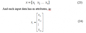
The average of all input data in each attribute is assumed to be zero. If this is not the case, the first change in attributes is to subtract each attribute from the average of that attribute in the total data, so that the average of each attribute in all data is zero.

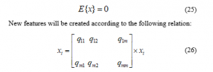
The j attribute of the i data changes with the following relation(In this relation, represents the j column of the Q matrix.)

Considering that the mean of the initial features is considered to be zero and also considering that the members of the Q matrix are fixed numbers, it can be said that the average of the new features that have coefficients of the original features will be equal to zero.

On the other hand, the covariance of the data is described by the following relation:

Since the average of the initial data is considered to be zero, as a result, the covariance of the primary data can be shown as follows:

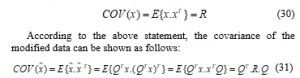
Since the data of all classes are expressed in the form of an x ​​matrix, it can be said that increasing the amount of covariance of the data mean that the data of different classes will be separated from each other. Therefore, the PCA task is defined to increase the covariance value of new data by selecting the appropriate values ​​for the members of the Q matrix.

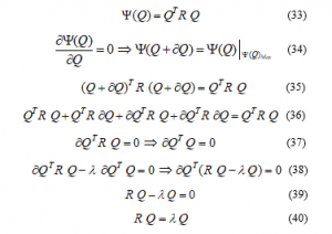
In the view of the above, the goal is to maximize the covariance of new features.

To solve the above equation, to find the values ​​of the Q matrix, use no change in the value of the function at the extreme points. So we will have:

After solving the above equation by MATLAB software, eigenvalues ​​(and eigenvectors in terms of eigenvalues) are arranged in descending order. New inputs (new features) can be calculated using the initial relation provided.

Instead of selecting all eigenvectors, it is sufficient to obtain a limited number of the best eigenvectors, so that, with minimal data loss, the dimensions of the data can be optimally reduced.

By evaluating the performance of each of the remaining features on the degree of classification, it is possible to eliminate the age features number 1, gender number 2, height number 3, and combination features 5,14,17. The accuracy of the classification maintains on 100%.

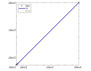
Figure 16: Neural network regression with 14 final features with 100% accuracy

5. Discussion

The accuracy obtained during each of the steps has shown in figure 17.

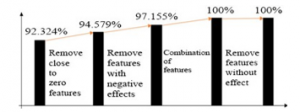
Figure 17: CCR extracted at various stages of feature reduction

In order to use the microcontroller for hardware implementation of the classifier neural network, the problem studied in this paper, in addition to accuracy, the study of occupied memory and performance speed is also of great importance.

Table 4 summarizes the accuracy, speed, and amount of memory occupied by the neural network in a microcontroller in each of the states described.

Table 4: Classification accuracy, execution time and memory occupied with microcontroller with the frequency 16MHz

Occupied memory	Execution time in microcontroller with the frequency 16MHz	Classification accuracy	Number of feature
11602	0.8243125	92.324%	279
6313	0.7830625	94.579%	150
4878	0.7678	97.155%	115
3932	0.714725	100%	20
2948	0.62425	100%	14

6. Conclusion

According to the noticeable increase of heart diseases and importance of the speed of getting the cardiac signals to diagnose and treat the diseases in time, by using artificial intelligent and Perceptron neural network during a multi- stage process by decreasing the number of characteristics, speed of getting the cardiac signals has maximized. During this process firstly the primary classification has done by 279 characteristics and 92.324% accuracy of Perceptron neural network has obtained. In next level, 35 characteristics with values near zero has omitted and second classification has done. The accuracy of the classification has increased from 92.324% to 94.579% and the number of characteristics has decreased from 279 to 150 by omitting the characteristics with values near zero. The effects of each characteristic on the amount of accuracy of neural network has investigated. Characteristics with undesirable effects has identified and the characteristics with undesirable effects on most networks has omitted. Number of characteristics decreased from 150 to 115 and by second classification, 97.155% accuracy obtained. In next level, to increase the accuracy of neural network with multiple classification of the characteristics, the number of characteristics has decreased from 115 to 20 and the accuracy of classification has increased from 97.155% to 100%. In final level, to minimize the number of characteristics and increase the speed of neural network as possible, by omitting ineffective or less effective characteristics in classification and keeping the accuracy on 100%, the number of characteristics has decreased from 20 to 14.

[1] The ECG signals received from the patient in the channels are DI, DII, DIII, aVR, aVL, aVF , V1 , V2, V3, V4, V5  and V6, respectively.

1. P. Christopher, MD. Cannon. “Cardiovascular disease and modifiable cardiometabolic risk factors”, Clinical Cornerstone, 8(3), pp. 11-28, 2007, doi:10.1016/s1098-3597(07)80025-1.
2. T.A. Gaziano, A. Bitton, Sh. Anand, S. Abrahams-Gessel, A. Murphy, “Growing Epidemic of Coronary Heart Disease in Low- and Middle-Income Countries”, Current Problems in Cardiology, vol. 35, no. 2,pp. 72–115 ,Feb 2010, doi:10.1016/j.cpcardiol.2009.10.002.
3. M. Naghavi, H. Wang, R. Lozano, A. Davis, X. Liang, M. Zhou, et al, “Global, regional, and national age–sex specific all-cause and cause-specific mortality for 240 causes of death, 1990–2013: a systematic analysis for the Global Burden of Disease Study 2013”, Lancet , 385 (9963), pp. 117-171, January 2015, doi:10.1016/S0140-6736(14)61682-2.
4. C.P. Cannon, “Cardiovascular disease and modifiable cardiometabolic risk factors”, Clinical Cornerstone, vol. 8, no. 3, pp. 11–28, 2007, doi:10.1016/s1098-3597(07)80025-1.
5. U. Zeymer, K. Schröder, U. Tebbe, et al. “Non-invasive detection of early infarct vessel patency by resolution of ST segment elevation in patients with thrombolysis for acute myocardial infarction. results of the angiographic substudy of the Hirudin for Improvement of Thrombolysis (HIT)-4 trial”, Eur Heart J , pp. 22-796, 2001, doi:10.1053/euhj.2000.2290.
6. S.G. Johnson, M.B. Farrell, A.M. Alessi, M.C. Hyun, “Nuclear Cardiology Technology Study Guide 2nd edition”, J. Nucl. Med. Technol. jnmt.116.175018 published ahead of print March 10, United States: SNMMI; pp. 17-19, 2016, doi:10.2967/jnmt.116.175018.
7. A S. Fauci, E. Braunwald, D L. Kasper, S L. Hauser, D L. Longo, J. Larry Jameson, J. Loscalzo, “Harrison Principles of Internal Medicine”, 15th ed. New York: McGraw-Hill; pp. 1386-99, 2001.
8. G. Hollander, V. Nadiminti, E. Lichstein, A. Greengart, M. Sanders, “Bundle branch block in acute myocardial infarction”, American Heart Journal, 105(5), pp. 738-743, 1983, doi:10.1016/0002-8703(83)90234-x.
9. J.J. Segura-Juarez, D. Cuesta-Frau, L. Samblas-Pena, M. Aboy, “A microcontroller-based portable electrocardiograph recorder”, IEEE Transactions on Biomedical Engineering, vol. 51 , no. 9 , Sep 2004, doi: 10.1109/TBME.2004.827539.
10. J. Francis, “ECG monitoring leads and special leads”, Indian Pacing and Electrophysiology Journal, vol. 16, no. 3, pp. 92-95, May–June 2016, doi:10.1016/j.ipej.2016.07.003.
11. P. D. Khandait, N. G. Bawane and S. S. Limaye, “Features extraction of ECG signal for detection of cardiac arrhythmias”, Proceedings of the National Conference on Innovative Paradigms in Engineering & Technology (NCIPET’2012), pp. 6-10, 2012, doi:10.1109/MAMI.2015.7456595.
12. D. Awasthi, S. Madhe, “Analysis of encrypted ECG signal in steganography using wavelet transforms”, Electronics and Communication Systems (ICECS), 2nd International Conference on, Coimbatore, pp. 718-723, 2015, doi:10.1109/ECS.2015.7125005.
13. K. Vanisree, J. Singaraju, “Decision support system for congenital heart disease diagnosis based on signs and symptoms using neural networks”, Int. J. Comput. Appl., vol. 19, no. 6, pp. 6-12, 2011, doi: 10.5120/2368-3115.
14. A. D. Dolatabadi, S. E. Z. Khadem, B. M. Asl, “Automated diagnosis of coronary artery disease (CAD) patients using optimized SVM”, Comput. Methods Programs Biomed, vol. 138, pp. 117-126, 2017, doi:10.1016/j.cmpb.2016.10.011.
15. K. Polat, S. shahan, S. Gunesh, “Automatic detection of heart disease using an artificial immune recognition system (AIRS) with fuzzy resource allocation mechanism and k-nn (nearest neighbour) based weighting preprocessing”, Expert Syst. Appl., vol. 32, no. 2, pp. 625-631, 2007, doi:10.1016/j.eswa.2006.01.027.
16. O. Mokhlessi, H. Masoudi Rad, N. Mehrshad, A. Mokhlessi, “Application of Neural Networks in Diagnosis of Valve Physiological Heart Disease from Heart Sounds”, American Journal of Biomedical Engineering, 1(1),pp. 26-34, 2011, doi:10.5923/j.ajbe.20110101.05.
17. P.Wallisch, M .Lusignan, M .Benayoun, T I .Baker, A S .Dickey, N G. Hatsopoulos: “MATLAB for Neuroscientists”, Second Ed, Academic Press, pp. 501-517, 2014, doi:10.1016/C2009-0-64117-9.
18. H. Yan, Y. Jiang, J. Zheng, C. Peng, Q. Li, “A multilayer perceptron-based medical decision support system for heart disease diagnosis”, Expert Systems with Applications, 30(2), pp. 272–281, 2005, doi:10.1016/j.eswa.2005.07.022.
19. L. Sharma, D.K. Yadav, A. Singh, “Fisher’s linear discriminant ratio based threshold for moving human detection in thermal video”, Infrared Physics & Technology, 78,pp. 118–128, 2016, doi:10.1016/j.infrared.2016.07.012.

(Click Here)

(Click Here)