1. Introduction

This paper is an extension of work originally presented in 3rd International Conference on Recent Developments in Control, Automation & Power Engineering (RDCAPE) [1].

With deregulation act in 2003, the reliability of the power system is enhanced in terms of availability and economics. The private sector intervened in the power generation and used the preexisting transmission system for distribution through pools. This resulted in overloading of lines to work under congestion, reaching their thermal and voltage limits [2]. The congestion resulted in huge amount of power losses thus effecting the economy of power transmission. There are two ways to relive the congested system. The cost-free method and the non-cost-free method. The cost-free method is one with no enhancement of operational cost. This is effectively achieved by incorporating Facts devices [3]. Power system is unevenly loaded. This results in inefficient output of the circuits. With uneven sharing of load through the lines, some lines become overloaded while others turn out to be under loaded. This distorts the voltage profile of the interconnected system [4]. FACTS being optimized for their respective parameters such as voltage angles, circuit reactance and voltage magnitudes, can be successfully incorporated in power system to modify the line parameters. This results in establishing a preferred bus and generator voltage profiles [5]. The system efficiency in terms of enhance loadability can be improved by suitably designing the controller of FACTS devices [6]. Maximum load on power system is industrial and domestic inductive load. Thus, there is significant voltage drop at these loads resulting in uneven voltage profile of system. Hence to reduce system inductive voltage drop, the inductive reactance has to be reduced in order to increase the power transfer capacity (PTC) of the system. The series FACTS device such as TCSC plays a vital role in achieving the reactance regulation [7]. To utilize the system at its maximum capacity together with power transmission economics, the transfer capacity of system must be enhanced to maximum value. System loadability improvement by increasing ATC value was achieved by an optimal power-flow-based model, for maximum power transfer by incorporating optimized FACTS control in the system [8]. Properly tuning FACT controller and its optimal location can reduce the system transmission losses and in return increases the power trans mitting capacity [9]. Different approaches were applied to optimize the location of fact devices. A number of heuristic methods like GA & BA were applied for optimal tuning of FACTS controller to enhance system ATC [10].

Further sensitivity index-based method for optimal allocation of FACTS devices such as SVC and TCSC was applied to enhance system power transfer capacity and hence ATC improvement [11]. The above-mentioned techniques resulted in ATC enhancement but this does not suffice the same improvements in other system parameters such as active power loss, reactive power loss and voltage profile regulation. The main objective of this paper is to develop a method with the incorporation of sensitivity index, ACPTDF together with an heuristic algorithm, Grey Wolf Optimization, (GWO) for minimizing the multi-objective function considered. This paper extends the area of implementation from a single objective of congestion management by ATC enhancement to a multi-objective of reducing active and reactive power losses as well as regulating the voltage profile of the system.

ATC of a power system is the power transfer capacity available above the maximum demand of the system, to be utilized for commercial activities between power suppliers and consumers. ATC is the back bone of any power system as it is directly influencing the power markets technically as well as economically [12]. The ATC of a power system can be enhanced by different methods and FACTS are very efficient in the same. The calculation of ATC can be done by different methods. A method was proposed to first calculate the reactive power flow and then by using PTDF as sensitivity factor ATC was calculated [13]. For enhancing the ATC value, generator terminal voltage and the output power can be worked within the defined security limits. ATC calculation and its values in power system database are therefore very crucial for the power market participants so as it can be used economically for industrial back up [14].

2. Related works

ATC for any system is the basis of restructuring of power system. Power system capability and its strength depends upon it ATC value [15].

The power system is interconnected, hence for enhancing the ATC of a particular system it is required that the power flow during the process must be technically very controlled. In other words, due to interconnection between different areas the ATC enhancement may result in change in power flow levels, resulting in unstable system. FACTS devices are quite a handful solution for this problem. Different types of FACTS devices use their specific properties to dynamically control the voltage magnitude, voltage angles and impedance of the lines while ATC enhancement is worked out. [16], [17].The FACTS devices are operated with the help of controllers. These controllers are either thyristor-controlled switch based or voltage source converter (VCS) based. These controllers helps to enhance the ATC while compensating for reactive power flow and reducing the active power losses [18]. A number of heuristic methods such as GA and PSO have been applied to program the controllers so as the FACTS device can compensate for reactive power and reduce active power loss while regulating the voltage profile of the system [19], [20].

Out of different FACTS devices TCSC is one of the most widely used device. ATC enhancement was done by applying continuation power flow (CPF) method taking thermal limits and voltage profile into account [21] .Other FACTS devices such as SSSC, STATCOM and UPFC have been modeled using heuristic methods like PSO and sensitivity index PTDF for ATC enhancement [22]. The controller of SSSC, UPFC and STATCOM have also been modeled by novel current based modeling for enhancing ATC instead of laying down new transmission line or rescheduling of generator [23]. ATC enhancement have also been done and compared by some more heuristic methods such as GA, PSO & FA under different contingency conditions [24].

3. Calculation of ATC

ATC in a power system can be calculated in numerous ways. Some methods are CPFM (continuous power flow method), linear approximation method etc. In this paper power sensitivity indices method is applied to calculate the ATC for standard IEEE 30 Bus system. The sensitivity factor applied here is Power Transfer Distribution Factor (PTDF). The PTDF can be of two types, DCPTDF and ACPTDF. Here we are applying ACPTDF for the calculation of ATC. ACPTDF determines the change in system power flow with the change in power transaction in some other line at steady state as well as under contingency conditions [25]. For a bilateral transaction between bus m and bus n. Here bus m is considered to sell power to bus n . The PTDF measures the change in real power flow of line i-j  due to bilateral transaction between m & n [26].

Mathematically,

where

P_mn is the power transaction between the bus m and n. Here bus m is considered to sell power to bus n. Bus n is considered to buy power in energy pooling system.

ΔP_ij is the change in power flow between bus i and j due to the bilateral transaction between bus m and n. This can be calculated as:

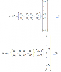
Now the power transfer in the line between buses i and j can be calculated for different values of PTDF as in equation (5)

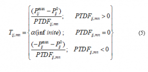
In equation (5)

 is active power flow limit of line i-j.

 is base case power flow in line i-j.

PTDF_{ij, mn} is the Power Transfer Distribution Factor for line i-j due to the exchange of active power between bus m and n.

Then ATC can be calculated as:

N_L is the total number of lines.

4. Reactive power flow

A fundamental aspect of the compensation and control of reactive power is its balance. The shunt capacitance of the transmission line yields reactive power proportional to the square of the voltage. Since the voltage must be kept within ± 5% of the rated voltage, the output or consumption of reactive power is relatively constant. The series inductance of the transmission line consumes reactive power proportional to the square of the current. Since the current varies from the duration of maximum demand to the duration of minimum demand, the reactive power consumption is also modified by the transmission line.

Figure number (1) shows the reactive power flow in the transmission system.

Figure 1: Reactive power flow in the Power system

The reactive power losses in the transmission line can be mathematically expressed as:

5. Modeling of TCSC

During the steady state, the compensator can freely change between reactance values according to its control. To avoid over-compensation of the line, limits are recommended for the TCSC reactance, given by the equation (7).

                                             

The proposed limit vary among different research works, but a tendency of capacitive factor greater than 50% of reactance of the line and inductive factor less than 25% of the inductance of the line is maintained.

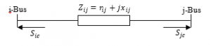
Figure 2: TCSC Power Injection Model [27]

In order to be used in power flow, the TCSC is modelled in form of line impedance with the built-in transformer reactance, in order to obtain the compensation scheme as shown in Figure (2)

The change in admittance is governed by the equation:

where,

 is the conductance of line ij before applying TCSC

 is the conductance of line ij after applying TCSC

 is the suceptance of line ij before applying TCSC

 is the suceptance of line ij after applying TCSC

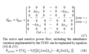
Equation (8) depicts that there is a variation of admittances by the application of the TCSC, so  the admittances matrix of the system will  be modified as indicated (13).

 

6. Objective Function

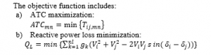
Thus, the multi-objective function can be written as:

7. Constraints and limits

While performing optimal power flow (OPF) on a system, there are certain parameters which are to be implemented with constraints and pre-defined limits as stated in the standard IEEE bus system appendix. Basically, there are two types of parameters. One parameter which involves expenses such as generation of power at generating end, . The other parameter which does not involve expenses are magnitude of voltages at generators,  and the transformer taps, .

The constraints in the system can be represented as summarized in Table number (1) below:

Table 1: Constraints incorporated in the system

Constraints	Equations
Power Balance (MW)
Power Balance (MVAr)	0
Generated Power (MW)
Generated Power (MVAr)
Bus Voltage Limits
Generator Voltage Limits
TCSC Reactance Limits

Where,

 represents real and reactive power generations at nth bus

 represents real and reactive power demand at nth bus

  represents real and reactive power injected at nth bus

 are voltage and resultant angle at nth bus

8. Grey Wolf Optimization

The heuristic technique implemented here to optimize the TCSC parameter is Grey Wolf Optimization (GWO). This technique is based on the well-organized social hierarchies of a pack of grey wolf. Grey wolf have a very typical and well defined hunting action. The hunting of prey is led by the most powerful alpha (a) wolf. The next hierarchy is taken by beta (b) wolf and the next one is taken by gamma(g) wolf. Rest of the wolfs in the pack are omega wolf. All the wolfs are guided by the alpha wolf. Hence the alpha wolf position in solution space is considered as the best solution, beta wolf, the next best and gamma wolf position the third best solution. The omega wolfs always follow the three best wolves throughout searching. GWO is divided into three processes, encircling, hunting and attacking the prey. Mathematically, the circling of prey can be symbolized as below [28].

where t is the current time,  is the vector representing location of the prey, __GW is a vector representing location of grey wolf, C & A are coefficient vectors and mathematically presented as:.

where “a”, is the error that is introduced in the system so as to avoid premature convergence of the algorithm. Its value is decreased from 2 to 0 through a series of iteration.

     represents arbitrary values between 0 and 1.

As the power system equations are highly non-linear and the solution can’t be realized by traditional methods so Grey wolf algorithm is simulated mathematically to locate the position of prey (solution). First three positions Alpha, Beta & gamma of wolf are best fitness values and position of omega wolves are updated with respect to the position of alpha, beta & gamma wolves and are mathematically be represented as:

This algorithm is applied in following steps:

1. The population of grey wolf is initialized with the initialization of initial parameters as:

• Size of the search space (defined by problem constraints)
• Number of search agents (here taken as 100)
• Vectors a, A & C
• Maximum number of iterations (100)

2. The wolves are randomly distributed in the pre-defined search space
3. The fitness value of each search agent is calculated and then indexed to get the best three fitness values. [from equation (24), (25) and (26)]
4. The three best positions are considered as best fitness values.
5. With respect to these three positions the fitness value of other wolfs are calculated.
6. Again the fitness values are sorted to get the updated positions of the wolfs [using equation (27)]
7. The fitness values are indexed and again first three values are considered as best fitness values.
8. The iterations are carried out till maximum iterations have reached or the fitness value become constant for defined number of iterations (in this paper equals to 50)

8.1 Pseudo code for GWO

Result: Bset value of fitness function

generate (X) / / Initialize the population of grey wolves

initialize Parameter (a, A, C);

evaluate X (0);

select new (Alpha, Beta, Delta, X (0));

for e = 1 to EVALMAX to do

for every Wolf l in Omega do

for i = 0 to DIM do

update Position (l, i); // Update current position

.         end for

adjust parameters (a, A, c); // adjust the algorithm   parameters

evaluate X (e + 1);

.       select new (Alpha, Beta, Delta, X (e + 1));

.       e = e + 1;

end for

end for

9. Methodology adopted

• • For ATC maximization (Without TCSC)

Figure (3) presents the sequence to calculate the ATC value without the application of TCSC. Here GWO is used only in NR with OPF only. While section 9.2 shows the steps followed to calculate ATC value using GWO optimized TCSC size and ACPTDF sorted location of TCSC. In the second case all the calculations are done once TCSC is located at a suitable position.

Figure 3: Process to calculate ATC without TCSC

• For Minimization of Reactive power loss (TQL)

For mminimization of power loss same two methods i.e. with and without TCSC are applied but with an objective to minimize reactive power loss only. With decreased value of reactive power loss, it can be observed that the ATC value is also decreased.

Here IEEE 30 bus system with six generators at bus number 1, 2, 5, 8, 11 and 13 is utilized for the application of the selected methodology. ACPTDF values are calculated for the transaction at a particular bus and its effect on power flow at all the other buses. Figure (4) gives the presentation of ACPTDF values when transactions are done between bus number 2 to 5 ad bus 2 to 26.

A number of evolutionary programming methods have been applied enhancement of ATC for a system but GWO turned to be one of the most suitable method to give optimized result for the chosen objective. Firefly algorithm have        been used for calculation of ATC with different FACTS devices [29] .GWO when used under similar circumstances with TCSC gave better results. Figure (5) gives a detailed presentation of the values of ATC and active power losses with both the methods are applied.

From fig (5) it can be depicted that while no FACTS device is connected in the system, the ATC value with GWO comes to be 12.18 MW significantly higher with that obtained for FA which comes to be 7.47 MW.

      Similarly, when the methods are applied for Total reactive power loss (TQL) reduction the power loss in case of GWO is 4.89 MW which is lesser then 5.01 MW obtained by applying FA. Moreover, the ATC value in case of TPL minimization is 10.54MW which is higher than 6.235 MW obtained by FA.

Figure 4: The ACPTDF values calculated for transaction between bus 2-5 and 2-26

10. Results and Analysis

The proposed optimization method is verified on 41 line, six generators, standard IEEE 30 BUS system [30] as shown in figure (6). Here except bus number 2, 5, 8, 11 and 13 where generators are connected, all the buses are considered as load bus. Also, all the generator buses are considered as seller buses while all other buses are the buyer buses.

Figure 5: Result comparison between GWO and FA without device

Figure.6:  Standard IEEE 30 bus system [30]

• ATC Maximization

The algorithm firstly applied for the objective of enhancement of ATC to reduce the congestion in the given system. The first step in this process is to calculate ATC with the help of ACPTDF. Figure (7) represents the effect of Generator at bus number 2 on ATC values of different parts of the system considered.

It can be seen that bus number 5 is nearest to generator and hence it has maximum value of ATC which equals 116.65 MW. On the other hand, bus number 26 is farthest from bus 2 so have a minimum value of ATC equal to 12.18 MW.

Figure number (8) represents the ATC distribution in the system due to generator at bus number 5 for all transactions. It can be well depicted that ATC value is largest, 184.56 MW for transaction between 5 to 2 and minimum, 12.16 MW for transaction between 5 to 26. The effect of generator at bus number 8 can be seen from figure number (9). This figure shows the distribution of ATC throughout the system for all transactions. Here it can be seen that maximum value of ATC, 70.41 MW is obtained at the line between bus 8-12 as bus 12 is nearest to bus 8. While the minimum value of ATC, 12.86 MW is obtained at line between 8-26.

Figure 7: ATC distribution in the system due to generator connected at bus number 2

      The effect of generator at bus number 11 on the distribution of ATC in the system for all transactions is shown in figure (10). It is clear from the figure that maximum value of ATC, 7.77 MW,

Figure 8: ATC distribution in the system due to generator connected at bus number 5

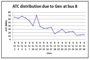
Figure 9: ATC distribution in the system due to generator connected at bus number 8

during all transactions is obtained at the line between seller bus 11 and the buyer bus 16. On the other hand, the minimum ATC value is obtained at the line between bus 11 and 26.

Figure 10: ATC distribution in the system due to generator connected at bus number 11

Effect of generator at bus number 13 is detailed in figure number (11). It is clear from the figure that maximum value of ATC, is obtained at line 13-7 and the minimum value of ATC, 8.89 MW is between bus 13 and 26 which is the farthest bus.

Figure 11: ATC distribution in the system due to generator connected at bus number 13

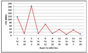
Figure 12: Variation of ATC values for all transactions due to generator at different buses

The maximum and the minimum ATC values can be represented in figure (12) for all generators.

It can be seen that the bus nearer to the generator bus are having higher ATC values. The lines 2-5, 5-2, 8-12, 11-16 and 13-7 are having higher ATC values as compared to their corresponding farther buses.After ATC being calculated for all generators and all buses, now the ATC value is to be calculated by incorporating TCSC. The position of TCSC is searched by ACPTDF where the value of ATC is maximum after being sorted by GWO for its optimized parameter. NR with OPF is performed to get the enhanced values of ATC after incorporating TCSC the result are being summarized in table number 2. From table no 2 the results for change in ATC and reactive power loss (TPL) can be predicted. The calculations were done by giving weightage to ATC maximization in equation number (19).. Together with the increase of ATC the power loss is also increased.

Table 2: ATC maximization consolidated results

Bus		ATC (MW)		TQL (MVAr)
SB	BB	Without TCSC	With TCSC	Without TCSC	With TCSC
2	5	116.65	120.75	82.33	30.5
	26	12.18	13.18	28.15	30.3
5	2	184.56	215.13	29.78	30.1
	26	12.26	13.45	28.48	30.7
8	12	70.41	74.056	28.26	30.4
	26	12.18	16.57	28.52	30.8
11	16	37.77	38.08	28.39	30.6
	26	6.09	8.01	29.24	31.3
13	7	34.67	36.89	27.56	29.6
	26	8.89	11.46	28.95	30.5

This increment in ATC value is higher when, percentage increase is compared from ATC enhancement by other optimization methods. In this case the percentage increase in ATP and TQL is shown in figure (13).

Figure 13: Percentage increment in ATC & TQL values with the incorporation of

TCSC

• Reactive Power loss minimization (TQL)

The second objective to minimize reactive power loss in the system is obtained by giving weightage to the TQL term in the objective function in equation (19).

Reactive power loss minimization results are depicted in table no.3. The table bears consolidated results when to reduce the reactive power losses is the objective. The table shows that reactive power losses are significantly reduced.

Table 3: TQL minimization consolidated results

Bus		ATC (MW)		TQL (MVAr)
SB	BB	Without TCSC	With TCSC	Without TCSC	With TCSC
2	5	116.65	90.67	28.33	25.36
	26	12.18	8.34	28.15	25.36
5	2	184.56	165.67	29.78	25.36
	26	12.26	9.45	28.48	25.36
8	12	70.41	45.89	28.26	25.36
	26	12.18	7.54	28.52	25.36
11	16	37.77	32.78	28.39	25.36
	26	6.09	6.03	29.24	25.36
13	7	34.67	32.43	27.56	25.36
	26	8.89	9.54	28.95	25.36

Together with reduction in reactive power losses, ATC value is also reduced. Again, in this case, because of the optimized TCSC location, reactive power loss is minimized.  The percentage reduction in reactive power loss is higher as compared to other evolutionary programming such as FA. Moreover, the reduction in ATC value with TCSC in line is less as compared to when other FACTS devices are used.  Figure (14) shows the percentage reduction in TQL and ATC with GWO optimized TCSC.

Table no 4: OPF result validation for ATC values in IEEE 30 bus system for far end bus

Bilateral Transactions Between Buses		ATC Values (MW)
From	To	FA [29]	GWO
2	26	7.6697	13.18
5	26	7.67154	13.45
8	26	7.81371	16.57
11	26	7.70317	8.01
13	26	7.66233	11.46

The OPF results for ATC maximization are validated with those obtained by Firefly Algorithm [29] and are presented in Table 4. The ATC value at the bus connected at the far end is low due to the transmission losses. The ATC value obtained by applying GWO is significantly higher as compared to that obtained by FA when far end values are compared. This validates GWO algorithm.

Fig no 14: Percentage decrement in TQL & ATC values with the incorporation of TCSC

11. Conclusion

In the current deregulated version of power system, where the expansion of the power system framework, due to economical and geographical constraints, can’t be expanded. Thus, the private market participants supplying their generation through the exiting lines, forcing the lines to work at their voltage and thermal limits hence creating congestion. To overcome this congestion, keeping the operational cost same, a versatile FACTS device, TCSC is tested here in the standard IEEE 30 bus system. TCSC parameters are optimised with the help of very versatile Grey Wolf Optimizer and the location of TCSC is optimized with the help of power system sensitivity factors, ACPTDF. The objectives of enhancing ATC value to reduce congestion in the system and to minimise reactive power loss are achieved. The objectives are achieved here within the prescribed voltage and thermal limit constraints. GWO being guided by the best fitness value (alpha wolf) as well as two more near to best fitness values i.e. beta   and gamma wolves. This ensures the speed of convergence. This optimiser uses three more variables a, A and C which ensures that GWO must not get stuck in the local minima and premature convergence. The ATC values for farther buses are quit low but this method optimised the TCSC parameter and its location such that the ATC value at far end should have higher values for greater utilization of lines and hence reduced the congestion. This paper utilised the pre-existing transmission lines for applying GWO and placing TCSC in the system to achieve the objectives of maximising ATC and reduction of reactive power loss to manage congestion in the system.

1. A. Gautam, P.R. Sharma, Y. Kumar, “Placement of TCSC applying Grey Wolf Optimization,” 313–318, 2019, doi:10.1109/RDCAPE47089.2019.8979016.
2. K.S. Verma, “Enhancement of Available Transfer Capability by the use of UPFC in Open Power Market,” 463–467, 2002.
3. M.B. K. Selvi, N. Ramaraj, “Total Transfer Capability Evaluation using Genetic Algorithms,” IE(I) Journal, 88, 60–64, 2007.
4. Y.H.S. and T.J. L. Gyugyi, Flexible AC Transmission Systems (FACTS), The Institutions of Electrical Engineers, Padstow, 1999.
5. N.G. Hingorani. and L. Gyugyi, Understanding FACTS, concepts and technology of flexible ac transmission systems, Wiley-IEEE Press, 2000.
6. S. Gerbex, R. Cherkaoui, A.J. Germond, “Optimal location of multi-type FACTS devices in a power system by means of genetic algorithms,” IEEE Transactions on Power Systems, 16(3), 537–544, 2001, doi:10.1109/59.932292.
7. A. Arzani, M. Jazaeri, Y. Alinejad-Beromi, “Available transfer capability enhancement using series FACTS devices in a designed multi-machine power system,” Proceedings of the Universities Power Engineering Conference, 4–9, 2008, doi:10.1109/UPEC.2008.4651434.
8. Y. Xiao, Y.H. Song, C. Liu, Y.Z. Sun, “Using FACTS Devices,” IEEE Transactions on Power Systems, 18(1), 305–312, 2003.
9. W. Ongsakul, P. Jirapong, “Optimal allocation of facts devices to enhance total transfer capability using evolutionary programming,” Proceedings – IEEE International Symposium on Circuits and Systems, 4175–4178, 2005, doi:10.1109/ISCAS.2005.1465551.
10. R. Mohamad Idris, A. Khairuddin, M.W. Mustafa, “A multi-objective bees algorithm for optimum allocation of FACTS devices for restructured power system,” IEEE Region 10 Annual International Conference, Proceedings/TENCON, 1–6, 2009, doi:10.1109/TENCON.2009.5395826.
11. J. Kumar, A. Kumar, W.Z. Gao, S. Yan, J. Wang, S. Gu, “ATC enhancement with SVC and TCSC using PTDF based approach in deregulated electricity markets,” Advanced Materials Research, 516–517, 1337–1341, 2012, doi: 10.4028/www.scientific.net/AMR.516-517.1337.
12. K. Mushfiq-Ur-Rahman, M. Saiduzzaman, M.N. Mahmood, M.R. Khan, “Calculation of available transfer capability (ATC) of Bangladesh power system network,” 2013 IEEE Innovative Smart Grid Technologies – Asia, ISGT Asia 2013, 1–5, 2013, doi:10.1109/ISGT-Asia.2013.6698716.
13. Ibraheem, N.K. Yadav, “Implementation of FACTS Device for Enhancement of ATC Using PTDF,” International Journal of Computer and Electrical Engineering, 3(3), 343–348, 2011, doi:10.7763/ijcee. 2011.v3.338.
14. P.W. Sauer, “Technical challenges of computing available transfer capability (ATC) in electric power systems,” Proceedings of the Hawaii International Conference on System Sciences, 5(2), 589–593, 1997, doi:10.1109/HICSS.1997.663220.
15. M.A. Khaburi, M.R. Haghifam, “A probabilistic modeling-based approach for Total Transfer Capability enhancement using FACTS devices,” International Journal of Electrical Power and Energy Systems, 32(1), 12–16, 2010, doi:10.1016/j.ijepes.2009.06.015.
16. S. Ahmad, F.M. Albatsh, S. Mekhilef, H. Mokhlis, “An approach to improve active power flow capability by using dynamic unified power flow controller,” 2014 IEEE Innovative Smart Grid Technologies – Asia, ISGT ASIA 2014, 249–254, 2014, doi:10.1109/ISGT-Asia.2014.6873798.
17. G. Hamoud, “Assessment of Available Transfer Capability of transmission systems,” IEEE Transactions on Power Systems, 15(1), 27–32, 2000, doi:10.1109/59.852097.
18. X. Jiang, X. Fang, J.H. Chow, A.A. Edris, E. Uzunovic, M. Parisi, L. Hopkins, “A novel approach for modeling voltage-sourced converter-based FACTS controllers,” IEEE Transactions on Power Delivery, 23(4), 2591–2598, 2008, doi:10.1109/TPWRD.2008.923535.
19. S. Panda, N.P. Padhy, “Comparison of particle swarm optimization and genetic algorithm for FACTS-based controller design,” Applied Soft Computing Journal, 8(4), 1418–1427, 2008, doi:10.1016/j.asoc.2007.10.009.
20. R. Eberhart, J. Kennedy, “New optimizer using particle swarm theory,” Proceedings of the International Symposium on Micro Machine and Human Science, 39–43, 1995, doi:10.1109/mhs.1995.494215.
21. T. Nireekshana, G. Kesava Rao, S. Siva Naga Raju, “Enhancement of ATC with FACTS devices using Real-code Genetic Algorithm,” International Journal of Electrical Power and Energy Systems, 43(1), 1276–1284, 2012, doi:10.1016/j.ijepes.2012.06.041.
22. K. Bavithra, S.C. Raja, P. Venkatesh, “Optimal setting of FACTS devices using particle swarm optimization for ATC enhancement in deregulated power system,” IFAC-Papers On Line, 49(1), 450–455, 2016, doi:10.1016/j.ifacol.2016.03.095.
23. S. Rahimzadeh, M.T. Bina, “Looking for optimal number and placement of FACTS devices to manage the transmission congestion,” Energy Conversion and Management, 52(1), 437–446, 2011, doi:10.1016/j.enconman.2010.07.019.
24. A. Gupta, A. Kumar, “ATC Determination with Heuristic techniques and Comparison with Sensitivity based Methods and GAMS,” Procedia Computer Science, 125(2017), 389–397, 2018, doi:10.1016/j.procs.2017.12.051.
25. A. Kumar, J. Kumar, “ATC determination with FACTS devices using PTDFs approach for multi-transactions in competitive electricity markets,” International Journal of Electrical Power and Energy Systems, 44(1), 308–317, 2013, doi:10.1016/j.ijepes.2012.07.050.
26. Shweta, V.K. Nair, V.A. Prakash, S. Kuruseelan, C. Vaithilingam, “ATC Evaluation in A Deregulated Power System,” Energy Procedia, 117, 216–223, 2017, doi:10.1016/j.egypro.2017.05.125.
27. G.A.N.S.B.S.S. N.M. Tabatabaei, “Optimal Location Of Facts Devices Using Adaptive Particle Swarm Optimization Mixed With Simulated Annealing,” International Journal on “Technical and Physical Problems of Engineering, 3(7), 60–70, 2011.
28. S. Mirjalili, S.M. Mirjalili, A. Lewis, “Grey Wolf Optimizer,” Advances in Engineering Software, 69, 46–61, 2014, doi:10.1016/j.advengsoft.2013.12.007.
29. M. Venkateswara Rao, S. Sivanagaraju, C. V. Suresh, “Available transfer capability evaluation and enhancement using various FACTS controllers: Special focus on system security,” Ain Shams Engineering Journal, 7(1), 191–207, 2016, doi:10.1016/j.asej.2015.11.006.
30. IEEE 30 Bus System. http://www.ee.washington.edu/research/pstca/pf30/pg_tca30bus.htm

(Click Here)

(Click Here)