1. Introduction

With rapid development of communication sciences especially satellites and cameras, the remote sensing images appeared with the importance of processing and dealing with this type of images (remote sensing images). One of these important image processing is classification which done by machine learning technology. Machine learning is one of the artificial intelligence branches that based on training computers using real data which result that computers will have good estimations as an expert human for the same type of data [1]. In 1959 the machine learning had a definition that “The machine learning is the field of study that gives computers the ability to learn without being explicitly programmed”, this definition was made by Arthur Samuel [2]. Where the declaration of machine learning problem was known as “a computer program is said to learn from experience E with respect to some task T and some performance measure P”, this declaration was made by Tom Mitchell in 1998 [3]. Deep learning is a branch of machine learning that depends on the Artificial Neural Networks (ANNs) which can be used in the remote sensing images classification [4]. In the recent years, with the appearance of the latest satellites versions and its updated cameras with high spectral and spatial resolution, the very high resolution (VHR) remote sensing images appeared. The redundancy pixels in the VHR remote sensing images can cause an over-fitting problem through training process where used the ordinary machine learning or ordinary deep learning in classification. So it must optimize the ANNs and have a convenient feature extraction from remote sensing images as a preprocessing before training the dataset [5-6]. The convolution Neural Networks (CNNs) is derived from the ANNs but its layers are not fully connected like the ANNs layers; it has an excited rapid advance in computer vision [7]. It is based on some blocks can applied on an image as filters and then extract convolution object features from this image, these features can be used in solving many of computer vision problems, one of these problems is classification [8]. The need of processing the huge data, which appeared with the advent of the VHR remote sensing images and its rapid development, produced the need of CNNs deep architectures that can produce a high accuracy in classification problems. It caused the appearance of the classic networks. There are many classic networks that are mentioned in the research papers which are established by researchers. However, this paper will inspect four of the well-known classic networks; the DenseNet 169, the NASNet Mobile, the VGG 16, and the ResNet 50 models. These four network models are used in the classification researches for the remote sensing images in many research papers. In [9], authors used the DenseNet in their research to propose a new model for improved the classification accuracy. In [10], authors used the DenseNet model to build dual channel CNNs for hyper-spectral images feature extraction. In [11], authors proposed a convolutional network based on the DenseNet model for remote sensing images classification. They build a small number of convolutional kernels using dense connections to produce a large number of reusable feature maps, which made the network deeper, but did not increase the number of parameters. In [12], authors proposed a remote sensing image classification method that based on the NASNet model. In [13], authors used the NASNet model as a feature descriptor which improved the performance of their trained network. In [14], authors proposed the RS-VGG classifier for classifying the remote sensing images which used the VGG model. In [15], authors proposed a combination between the CNNs algorithms outputs, one of these algorithms outputs is the outputs of the VGG model, and then constructed a representation of the VHR remote sensing images for resulting VHR remote sensing images understanding. In [16], authors used the pre-trained VGG model to recognize the airplanes using the remote sensing images. In [17], authors performed a fully convolution network that based on the VGG model for classifying the high spatial resolution remote sensing images. They fine-tuned their model parameters by using the ImageNet pre-trained VGG weights. In [18], authors proposed the use of the ResNet model to generate a ground scene semantics feature from the VHR remote sensing images, then concatenated with low level features to generate a more accurate model. In [19], authors proposed a classification method based on collaborate the 3-D separable ResNet model with cross-sensor transfer learning for hyper-spectral remote sensing images. In [20], authors used the ResNet model to propose a novel method for classifying forest tree species using high resolution RGB color images that captured by a simple grade camera mounted on an unmanned aerial vehicle (UAV) platform. In [21], authors proposed an aircraft detection methods based on the use of the deep ResNet model and super vector coding. In [22], authors proposed a remote sensing image usability assessment method based on the ResNet model by combining edge and texture maps.
The aim of this paper is to compare the using of the deep convolution models classic networks in classifying the remote sensing images. The used networks in this comparison are the DenseNet 196, the NASNet Mobile, the VGG 16, and the ResNet 50 models. This comparative study is based on inspecting the learning curves for the training and validation loss and training and validation accuracy through training process for each epoch. This inspection is done to determine the efficient of the model hyper-parameters selection. It is based also on calculating the overall accuracy (OA) of these four models in remote sensing images classification to determine the learning model performance. There are two use datasets in this comparative; the UC Merced Land use dataset and the SIRI-WHU dataset.
The rest of this paper is organized as follow. Section 2 gives the methods. The experimental results and setup are shown in section 3. Section 4 presents the conclusions followed by the most relevant references.

The Methods

In this section the used models, in this comparative study, will explained with its structures. The classic networks that used in this study will illustrated in brief as literature review, ending with how to assess the performance of the learning models.

The Used Models

The feature extraction of remote sensing images is provided an important basis in remote sensing images analysis. So, in this study the deep classic convolution networks outputs considered as the main features that extracted from the remote sensing images. In these four networks, we used the ImageNet pre-trained weights because the train of new CNNs models requires a large amount of data. We transfer learning, add full connected (FC) layers with the output layer containing neurons number that equal the dataset classes number (21 for the UC Merced land use dataset and 12 for the SIRI-WHU dataset), and then train these (FC) layers.
In the DenseNet 169 model we transfer learning to the last hidden layer before the output layer (has 1664 neurons) and get the output of this network with the ImageNet pre-trained weights, then adding FC layer (output layer) with softmax activation.
In the NASNet Mobile model we transfer learning to the last hidden layer before the output layer (has 1056 neurons) and get the output of this network with the ImageNet pre-trained weights, then adding FC layer (output layer) with softmax activation.
In the VGG 16 model we transfer learning to the output of last max pooling layer (has shape 7, 7, 512) in block 5 that before the first FC layer and get the output of this network with the ImageNet pre-trained weights, then adding FC layer (output layer) with softmax activation.
In the ResNet 50 model we transfer learning to the last hidden layer before the output layer (has 2048 neurons) and get the output of this network with the ImageNet pre-trained weights, then adding FC layer (output layer) with softmax activation.

The Convolution Neural Networks (CNNs)

The CNNs are taken from the ANNs with exception that it is not fully connected layers. The CNNs are the best solution for computer vision which based on some of filters to reduce the image height and width and increase the number of channels together, then processing the output with full connected neural network layers (FCs) which reduce the input layer neurons, reduce training time, and increase the training model performance [23-25]. These filters values are initialized with many random functions which can be optimized.

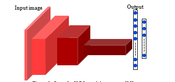Figure 1: One of a CNNs model structures [25]

The filters design is based on the use of self-intuition as with ANNs structure design and learning hyper-parameters coefficient choice, which increasing the difficulty to reach the best solution for the learning problems [25]. Figure 1 shows an example of a CNNs model structure [24].

The DenseNet Model

In 2017, the DenseNets was proposed in the CVPR 2017 conference (Best Paper Award) [26]. They started from attempted to build a deeper network based on an idea that if the convolution network contains shorter connections between its layers close to the input and those close to the output, this deep convolution network can be more accurate and efficient to train. Other than the ResNet model which adds a skip-connection that bypass the nonlinear transformation, the DenseNet add a direct connection from any layer to any subsequent layer. So the l^th layer receives the feature-maps of all former layers x_0 to x_(l-1) as (1) [26].

where [x_0,〖 x〗_1,…,〖 x〗_(l-1) ] refers to the spectrum of the feature-map produced in the layers 0,1,2,…,l-1.
Figure 2 shows the 5-layers dense block architecture and Table 1 shows the DenseNet 169 architectures for ImageNet. [26].

Table 1: the DenseNet 169 model architectures for ImageNet [26]
Layers	Output Size	DenseNet 169
Convolution	112 112	7 7 conv, stride 2
Pooling	56 56	3 3 max pool, stride 2
Dense Block (1)	56 56
Transition Layer (1)	56 56	1 1 conv
	28 28	2 2 average pool, stride 2
Dense Block (2)	28 28
Transition Layer (2)	28 28	1 1 conv
	14 14	2 2 average pool, stride 2
Dense Block (3)	14 14
Transition Layer (3)	14 14	1 1 conv
	7 7	2 2 average pool, stride 2
Dense Block (4)	7 7
Classification Layer	1 1	7 7 global average pool
	1000	1000D fully-connected, softmax

The NASNet Model

In 2017, the NASNet (Neural Architecture Search Net) model was proposed in the ICLR 2017 conference [27]. They used the recurrent neural networks (RNNs) to generate the model description of the neural networks and trained the RNNs with reinforcement learning to improve the accuracy of the generated architectures on a validation set. The NASNet model is based on indicting the previous layers that elected to be connected by adding an anchor point which has N-1 content-based sigmoid using (2). Figure 3 shows one block of a NASNet convolutional cell [27].

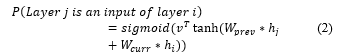
where h_j refers to the hidden state of the controller at anchor point for the j^th layer and j=[0,1,2,…,N-1].

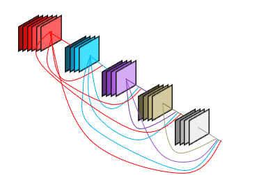Figure 2: The 5 layers Dense block architecture [26]

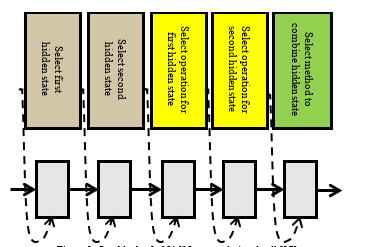Figure 3: One block of a NASNet convolutional cell [27]

The VGG Model

In 2015, the VGG network was proposed in the ICLR 2015 conference [28]. They began with investigated the effect of the convolution network depth on its accuracy in the large-scale images. Through they evaluated the deeper networks architecture using (3×3) convolution filters, they showed that an expressive growth on the prior-art configurations can be achieved by pushed the depth to 16-19 weight layers. Table 2 shows the VGG 16 model architectures for the ImageNet [28].

Table 2: The VGG 16 model architectures for ImageNet [28]
Block	Layers	Output Size	VGG 16
Input		224 224 3
Block 1	Convolution	224 224 64	3 3 conv 64, stride 1
	Convolution	224 224 64	3 3 conv 64, stride 1
	Pooling	112 112 64	2 2 max pool, stride 2
Block 2	Convolution	112 112 128	3 3 conv 128, stride 1
	Convolution	112 112 128	3 3 conv 128, stride 1
	Pooling	56 56 128	2 2 max pool, stride 2
Block 3	Convolution	56 56 256	3 3 conv 256, stride 1
	Convolution	56 56 256	3 3 conv 256, stride 1
	Convolution	56 56 256	3 3 conv 256, stride 1
	Pooling	28 28 256	2 2 max pool, stride 2
Block 4	Convolution	28 28 512	3 3 conv 512, stride 1
	Convolution	28 28 512	3 3 conv 512, stride 1
	Convolution	28 28 512	3 3 conv 512, stride 1
	Pooling	14 14 512	2 2 max pool, stride 2
Block 5	Convolution	14 14 512	3 3 conv 512, stride 1
	Convolution	14 14 512	3 3 conv 512, stride 1
	Convolution	14 14 512	3 3 conv 512, stride 1
	Pooling	7 7 512	2 2 max pool, stride 2
FC		4096
FC		4096
Output		1000, softmax

The VGG network is a deeper convolution network that trained on the ImageNet dataset. The input images of this network is (224×244×3). This network consists of five convolution blocks, each block is containing convolution layers and pooling layer, then ending with two FC layers (each layer has 4096 neurons) then the output layer with softmax activation. The VGG network doesn’t contain any layers connections or bypasses such as the ResNet, the NASNet or the DenseNet models, and at the same time gives high classification accuracy with the large scale images [28].

The ResNet Model

In 2016, the ResNet was proposed in the CVPR 2016 conference [29]. They combined the degradation problem by introducing a deep residual learning framework. Instead of intuiting each few stacked layers directly fit a desired underlying mapping. The ResNet is based on skip connections between deep layers. These skip connections can skipping one or more layers. The outputs of these connections are added to the outputs of the network stacked layers as (3) [29].

where H(x) is the final block output, x is the output of the connected layer, and F(x) is the output of the stacked networks layer in the same block.
Figure 4 shows the ResNet one building block. Tables 3 shows the ResNet 50 network architectures for the ImageNet [29].

Table 3: the ResNet 50 model architectures for ImageNet [29]
Layers	Output Size	ResNet 50
Conv 1	112 112	7 7 conv 64, stride 2
Conv 2_x	56 56	3 3 max pool, stride 2
Conv 3_x	28 28
Conv 4_x	14 14
Conv 5_x	7 7
Classification Layer	1 1	7 7 global average pool
	1000	1000D fully-connected, softmax

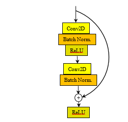Figure 4: The ResNet building block [29]

The Performance Assessment

There are many matrices for gauge the performance of the learning models. One of these is the OA. The OA is the main classification accuracy assessment [30]. It is measure the percentage ratio between the corrected estimation test data objects and all the test data objects in the used dataset. The OA is calculated using (4) [30, 31].

The learning curves for the loss and the accuracy are very important indicator for determining the power of learning models through training process by using the corrected hyper-parameters [32]. By using these curves, you can determine if a problem exist on your learning model such as the over-fitting or the under-fitting problems. These curves represent the calculation of the loss and the accuracy values for the learning model at each epoch through the training process using training and validation data [32, 33].

Experimental Results and Setup

This comparative study is based on calculating the OA and plotting the learning curves to determine the power of the used hyper-parameter to achieved the better learning model performance. The UC Merced Land use dataset and the SIRI-WHU dataset are the used datasets in this study. The details of these datasets will introduce in this section and then the experiments setup details and the results.

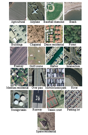Figure 5: Image examples from the 21 classes in the UC Merced land use dataset [34]

The UC Merced Land Use Dataset

The UC Merced Land use dataset is a collection of remote sensing images which has been prepared in 2010 by the University of California, Merced [34]. It consists of 2100 remote sensing images divided into 21 classes with 100 images for each class. These images were manually extracted from large images from the USGS National Map Urban Area Imagery collection for various urban areas around the USA. Each image in this dataset is Geo-tiff RGB image with 256×256 pixels resolution and 1 square foot (0.0929 square meters) spatial resolution [34]. Figure 5 shows image examples from the 21 classes in the UC Merced land use dataset [34].
The SIRI-WHU Dataset
The SIRI-WHU dataset is a collection of remote sensing images which the authors of [35] used this dataset in their classification problem research in 2016. This dataset consists of two versions that must complete each other. The total images in this dataset are 2400 remote sensing images divided into 12 classes with 200 images for each class. These images were extracted from Google Earth (Google inc.) and mainly cover urban areas in China. Each image in this dataset is Geo-tiff RGB image with 200×200 pixels resolution and 2 square meters (21.528 square foot) spatial resolution [35]. Figure 6 shows image examples with 12 classes in the SIRI-WHU dataset [35].

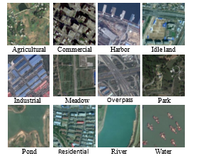Figure 6: Image examples from the 12 classes in the SIRI-WHU dataset [35].

The Experimental Setup

The aim of this paper is to present a comparative study of using the classic networks for classifying the remote sensing images. This comparison is based on plotting the learning curves for the loss and the accuracy values, with every epoch, that be calculated through training process for the training and the validation data to determine the efficiency of the hyper-parameters values. The comparison is also based on the OA to assess each model performance. The used datasets in this study are the UC Merced land use dataset and the SIRI-WHU dataset where their details are stated in sections 3.1 and 3.2. All tests were performed using Google-Colab. The Google-Colab is a free cloud service hosted by Google inc. to encourage machine learning and artificial intelligence researches [36]. It is acts as a virtual machine (VM) that using 2-cores Xeon CPU with 2.3 GHz, GPU Tesla K80 with 12 GB GPU memory, 13 GB RAM, and 33GB HDD with Python 3.3.9. The maximum lifetime of this VM is 12 hours and it will be idled after 90 minutes time out [37]. Performing tests has been done by connecting to this VM online through ADSL internet line with 4Mbps communication speed. This connection was done using an Intel® coreTMi5 CPU M450 @2.4GHz with 6 GB RAM and running Windows 7 64-bit operating system. This work is limited by used the ImageNet pre-trained weights because the train of new CNNs models needs a huge amount of data and more sophisticated hardware, this is unlike the lot of needed time consumed for this training process. The other limitation is that the input images shape is mustn’t less than 200×200×3 and not greater than 300×300×3 because of the limitations of the pre-trained classic networks. The preprocessing step according to each network requirements is necessary to get efficient results; it must be as done on ImageNet dataset before training the models and produce the ImageNet pre-trained weights. The ImageNet pre-trained weights classic networks that used in this paper have input shape (224, 224, 3) and output layers 1000 nodes according to the ImageNet classes (1000 classes) [38, 39]. So, it must perform modifications on the learning algorithms that used these networks to be compatible with the used remote sensing images datasets as stated in section 2.1. The data in the used datasets were divided into 60% training set, 20% validation set, and 20% test set before training the last FC layers in each network model. The training process, using the training set and the validation set, is done for the model with a supposed number of epochs to determine the number of epochs that achieved the minimum validation loss. Thus, we consider that the assembling of the training set and the validation set are the new training data and then retrain the model with this new training set and the predetermined number of epochs that achieved the minimum validation loss. Finally test the model using the test set. It must be notice that, the learning parameters values, such as learning rate and batch size, were determined by intuition with taking in consideration the learning parameters values that used through training these models with the ImageNet dataset through producing the ImageNet pre-trained weights [26-29], where the used optimizer, the number of epochs, the additional activation and regularization layers, and the dropout regularization rates were determined by iterations and intuition. The classifier models are built using python 3.3.9, in addition to the use of the Tensorflow library for the preprocessing step and the Keras library for extracting features, training the last FC layers, and testing the models.
In the DenseNet 196 model, the image resizing was done on the dataset images to have shape (224, 224, 3) to be compatible with the pre-trained DenseNet 196 model input shape, perform transfer learning to the 7×7 global average pooling layer that above the 1000D FC layer, and then add a FC layer, which has number of neurons equal to the used dataset classes, with softmax activation layer. The last layer weights were retrained with learning rate = 0.001, Adam optimizer and batch size = 256 with 100 epochs. The normalization preprocessing must be done on the dataset images before using on the DenseNet 169 model. Figure 7 shows the flow chart of the experimental algorithm that used the DenseNet 169 model.
In the NASNet Mobile model, the image resizing was done on the dataset images to have shape (224, 224, 3) to be compatible with the pre-trained NASNet Mobile model input shape, perform transfer learning to the 7×7 global average pooling layer that above the 1000D FC layer, add a ReLU activation layer, dropout regularization layer with rate 0.5, and then adding a FC layer, which has number of neurons equal to the used dataset classes, with softmax activation layer. The last layer weights were retrained with learning rate = 0.001, Adam optimizer, and batch size = 64 with 200 epochs. The normalization preprocessing must be done on the dataset images before using on the NASNet Mobile model. Figure 8 shows the flow chart of the experimental algorithm that used the NASNet Mobile model.

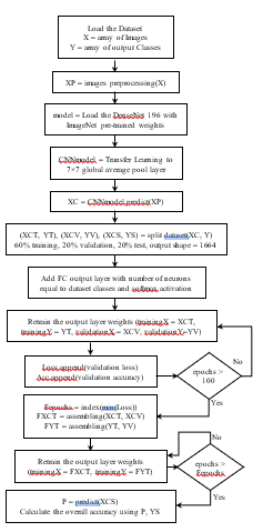Figure 7: The flow chart of the experimental algorithm that used the DenseNet 169 model

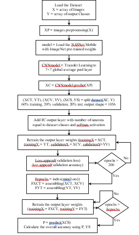Figure 8: The flow chart of the experimental algorithm that used the NASNet Mobile model

In the VGG 16 model, the image resizing was done on the dataset images to have shape (224, 224, 3) to be compatible with the pre-trained VGG 16 model input shape, perform transfer learning to the 2×2 max pooling layer in block 5, flatten the pooling layer output, add a ReLU activation layer, dropout regularization layer with rate 0.77, and then add a FC layer, which has number of neurons equal to the used dataset classes, with softmax activation layer. The last layer weights were retrained with learning rate = 0.001, Adam optimizer, and batch size = 64 with 100 epochs. The image conversion to the BGR mode preprocessing must be done on the dataset images before using on the VGG 16 model. Figure 9 shows the flow chart of the experimental algorithm that used the VGG 16 model.

 

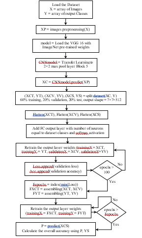Figure 9: The flow chart of the experimental algorithm that used the VGG 16 model

In the ResNet 50 model, the image resizing was done on the dataset images to have shape (224, 224, 3) to be compatible with the pre-trained ResNet 50 model input shape, perform a transfer learning to the 7×7 global average pooling layer that above the 1000D FC layer, and then add a FC layer, which has number of neurons equal to the used dataset classes, with softmax activation layer. The last layer weights were retrained with learning rate = 0.1, Adam optimizer, and batch size = 64 with 200 epochs. The image conversion to the BGR mode preprocessing must be done on the dataset images before using on the ResNet 50 model. Figure 10 shows the flow chart of the experimental algorithm that used the ResNet 50 model.

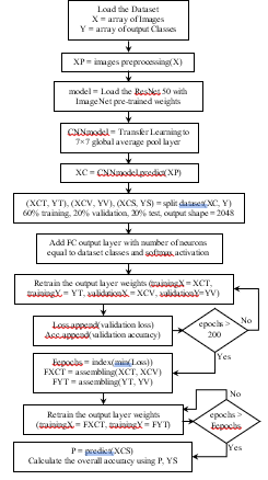Figure 10: The flow chart of the experimental algorithm that used the ResNet 50 model

The Experimental Results

With the use of the stated convolution models in this study for classifying remote sensing images, through the training process we used the training data (60% from the used dataset) and the validation data (20% from the used dataset). Figure 11 shows the loss and the accuracy learning curves respectively for training the DenseNet 169 model, (a) for using the UC Merced land use dataset and (b) for using the SIRI-WHU dataset. Figure 12 shows the loss and the accuracy learning curves respectively for training the NASNet Mobile model, (a) for using the UC Merced land use dataset and (b) for using the SIRI-WHU dataset. Figure 13 shows the loss and the accuracy learning curves respectively for training the VGG 16 model, (a) for using the UC Merced land use dataset and (b) for using the SIRI-WHU dataset. Figure 14 shows the loss and the accuracy learning curves respectively for training the ResNet 50 model, (a) for using the UC Merced land use dataset and (b) for using the SIRI-WHU dataset.

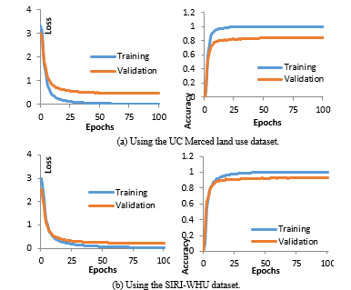Figure 11: The loss and the accuracy learning curves for training the DenseNet 169 model.

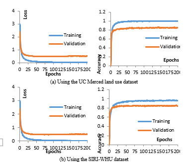Figure 12: The loss and the accuracy learning curves for training the NASNet Mobile model.

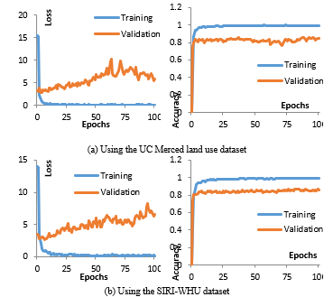Figure 13: The loss and the accuracy learning curves for training the VGG 16 model.

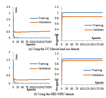Figure 14: The loss and the accuracy learning curves for training the ResNet 50 model.

From the learning curves it can be determine the number of epochs that achieved the minimum validation loss in each model from the four models that discussed in this study. So, we consider that the training data and the validation data, 80% from dataset, are the new training data. Then, we repeat the same training process for each model with the same hyper-parameters values and the both datasets, and then calculate the OA using the predictions of the test data, 20% from the training set, to assess the performance of each model. Table 4 and figure 15 show the OA for each model using the both datasets.
Table 4: The OA for each model using the both datasets

Table 4: The OA for each model using the both datasets
	The UC Merced land use Dataset	The SIRI-WHU Dataset
The DenseNet 169 model	0.91	0.933
The NASNet Mobile model	0.876	0.896
The VGG 16 model	0.902	0.929
The ResNet 50 model	0.924	0.956

As shown from these results, the ResNet 50 model had the higher OA in this comparative study where the NASNet Mobile model had the lowest OA. In the other hand the OA for the DenseNet 169 model had little higher OA than the VGG 16 model. The use of the SIRI-WHU dataset had higher OA than the use of the UC Merced land use dataset. These results illustrated that the OA had an opposite relation with the dataset image resolution and the dataset number of classes, so the use of the SIRI-WHU dataset which has 12 classes, image resolution 200×200 pixels, and spatial resolution 2 square meters gave higher OA than the use of the UC Merced land use dataset which has 21 classes, image resolution 256×256 pixels, and spatial resolution 0.0929 square meter. The deeper convolution networks give considerable accuracy but the connections between layers may have another influence. The VGG 16 model gave good OA so it had efficient results but its learning curves had some degradation in its validation curves and near to the over-fitting in its training curves. So it may give better results with some additional researches that adjust the optimizations and regularization hyper-parameters. In the other hand the ResNet 50 model, that gave the higher OA in this study, had good learning curves with some little over-fitting. So, with more research and adjusting the regularization hyper-parameters, it is not easy to achieve higher results using this model without any major development. The ResNets are based on the skip layers connections so the layer connections can raise the classification accuracy. The DenseNets may have more connections but still the ResNet 50 model had the higher OA in this comparative study. The NASNets models have layers connections but not more as the DenseNets models, these connections only to determine the previous layer, so its results are low compared with other models in this study. In the other hand the NASNet’s model learning curves are good, no degradation and no over-fitting, but with increasing the epochs the validation loss may be raised, so it must have an attention observed for epochs and validation curves through training this model. As a total the deeper convolution networks may give better accuracies but the deeper networks that have layers connections may give the best accuracies.

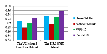Figure 15: The OA for each model using the both datasets

Conclusions

This paper presented a comparative study for the use of the deep convolution models classic networks in classifying the remote sensing images. This comparison illustrated that what the classic network was more accurate for classifying the VHR remote sensing images. The used classic networks in this study were the DenseNet 169, the NASNet Mobile, the VGG 16, and the ResNet 50 models. There were two used datasets in this study; the UC Merced land use dataset and the SIRI-WHU dataset. This comparison was based on the learning curves to check that how much effectiveness of the hyper-parameters values selection and the overall accuracy to assess the classification model performance. This comparison illustrated that the ResNet 50 model was more accurate than other models that stated in this study, which the overall accuracy of the DenseNet 169 model was little higher than the VGG 16 model. The NASNet Mobile model had the lowest OA in this study. The learning curves elucidated that the adjustment of the hyper-parameters of the VGG 16 model can lead to better overall accuracy where it is not easy to achieve better overall accuracy in the ResNet 50, the DenseNet 169 and the NASNet Mobile models without major developments in these models. The overall accuracy had an opposite relation with the remote sensing images resolution (pixel or spatial) and the number of dataset classes.
In the future, the FC layers can be replaced by other classifiers, and then train these models.

Conflict of Interest

The authors declare no conflict of interest.

1. O. Afolabi, “Commuters Perception and Preferences on The Bus Rapid Transit in Lagos State,” JORIND, 14(2), 2016.
2. J. Cao, X. Cao, C. Zhang, X. Huang, “The gaps in satisfaction with transit services among BRT, metro, and bus riders: Evidence from Guangzhou,” Journal of Transport and Land Use, 97–109, 2015, doi:10.5198/jtlu.2015.592.
3. D. Darwis, Fatmawati, Nasrulhaq, “Hubungan Kualitas Pelayanan dengan Kepuasan Masyarakat Pengguna Bus Rapid Transit (BRT) Maminasata,” Administrasi Publik, 3, 2017.
4. J.M. Bunker, “High volume bus stop upstream average waiting time for working capacity and quality of service,” Public Transport, 10(2), 311–333, 2018, doi:10.1007/s12469-018-0179-1.
5. M. Islam, M. Brussel, A. Grigolon, T. Munshi, “Ridership and the Built-Form Indicators: A Study from Ahmedabad Janmarg Bus Rapid Transit System (BRTS),” Urban Science, 2(4), 95, 2018, doi:10.3390/urbansci2040095.
6. D. Oviedo, L. Scholl, M. Innao, L. Pedraza, “Do Bus Rapid Transit Systems improve accessibility to job opportunities for the poor? The case of Lima, Peru,” Sustainability (Switzerland), 11(10), 2019, doi:10.3390/su11102795.
7. D.A. Rodriguez, C.E. Vergel-Tovar, “Urban development around bus rapid transit stops in seven cities in Latin-America,” Journal of Urbanism, 11(2), 175–201, 2018, doi:10.1080/17549175.2017.1372507.
8. E. Saputra, C. Widyasmara, “The effect of urban spatial structure on rapid bus transit services in Yogyakarta and Surakarta, Indonesia: A comparative study of the Trans Jogja and the Batik Solo Trans,” Geografia – Malaysian Journal of Society and Space, 10(2), 46–58, 2014.
9. S. Tao, J. Corcoran, I. Mateo-Babiano, D. Rohde, “Exploring Bus Rapid Transit passenger travel behaviour using big data,” Applied Geography, 53, 90–104, 2014, doi:10.1016/j.apgeog.2014.06.008.
10. L. Prayogi, “The Influence of Bus Rapid Transit System on Urban Development: An Inquiry to Boston and Seoul BRT Systems,” International Journal of Built Environment and Scientic Research, 1(1), 1–8, 2017.
11. A. Koling, W.-B. Zhang, K. Zhou, H. Meng, Bus Rapid Transit ( BRT ) Toolbox: Assessing Person Throughput to Measure Transportation Impacts for BRT Projects, 2018.
12. S. Tabassum, S. Tanaka, F. Nakamura, “Improving Access considering Commuters ’ Perception ( A Case Study of Lahore BRT ) Keywords:,” International Journal of Innovative Research in Engineering and Management (IJIREM), 3(4), 283–289, 2016.
13. M. Woldeamanuel, C. Olwert, “The Multimodal Connectivity at Bus Rapid Transit (BRT) Stations and the Impact on Ridership,” Journal of the Transportation Research Forum, 55(1), 87–102, 2016, doi:10.5399/osu/jtrf.55.1.4340.
14. B. Ferhan, X. Zhou, “Drivers , Barriers and Implementation of Social Sustainable in Supply Chain A qualitative study of SMEs,” 1–83, 2016.
15. S. Nasrin, “Acceptability of Bus Rapid Transit ( BRT ) to Commuters in Dhaka,” 2015.
16. H.I. Okagbue, M.O. Adamu, S.A. Iyase, E.A. Owoloko, On the Motivations and Challanges Faced by Commuters Using Bus Rapid Transit in Lagos, Nigeria, The Social Sciences, 10(6), 696–701, 2015, doi:10.3923/sscience.2015.696.701.
17. J. Dubé, F. Des Rosiers, M. Thériault, P. Dib, “Economic impact of a supply change in mass transit in urban areas: A Canadian example,” Transportation Research Part A: Policy and Practice, 45(1), 46–62, 2011, doi:10.1016/j.tra.2010.09.002.
18. J.B. Ingvardson, O.A. Nielsen, “Effects of new bus and rail rapid transit systems–an international review,” Transport Reviews, 38(1), 96–116, 2018, doi:10.1080/01441647.2017.1301594.
19. E. Adewumi, D. Allopi, “An Appropriate Bus Rapid Transit System,” International Journal of Science and Technology Volume 3 No. 4, 3(4), 248–254, 2014.
20. A.P. Ajayi, “Assessment of the Influence of Lagos Bus Rapid Transit Scheme (BRT-Lite) on Road Traffic Crashes (RTC) on Lagos Mainland-Island Corridor,” The Open Transportation Journal, 11(1), 102–109, 2017, doi:10.2174/1874447801711010102.
21. A. Nikitas, M. Karlsson, “A Worldwide State-of-the-Art Analysis for Bus Rapid Transit: Looking for the Success Formula,” Journal of Public Transportation, 18(1), 1–33, 2015, doi:10.5038/2375-0901.18.1.3.
22. A. Mishra, S.A.S.A. Kumar, P. Pradeep, “Study of Bus Rapid Transit system In Respect to Growing Cities of India,” Nternational Journal of Engineering Research & Technology (IJERT), 2(10), 1378–1383, 2013.
23. M. Poku-Boansi, G. Marsden, “Bus rapid transit systems as a governance reform project,” Journal of Transport Geography, 70(June), 193–202, 2018, doi:10.1016/j.jtrangeo.2018.06.005.
24. S.R. Majumdar, “The case of public involvement in transportation planning using social media,” Case Studies on Transport Policy, 5(1), 121–133, 2017, doi:10.1016/j.cstp.2016.11.002.
25. E. Cascetta, F. Pagliara, “Public Engagement for Planning and Designing Transportation Systems,” Procedia – Social and Behavioral Sciences, 87, 103–116, 2013, doi:10.1016/j.sbspro.2013.10.597.
26. K. Rangarajan, S. Long, A. Tobias, M. Keister, “The role of stakeholder engagement in the development of sustainable rail infrastructure systems,” Research in Transportation Business and Management, 7, 106–113, 2013, doi:10.1016/j.rtbm.2013.03.007.
27. N. Hassen, P. Kaufman, “Examining the role of urban street design in enhancing community engagement: A literature review,” Health and Place, 41, 119–132, 2016, doi:10.1016/j.healthplace.2016.08.005.
28. J.R. Gardner, R. Rachlin, H.W.A. Sweeney, A. Sweeny, H.W. Allen, Handbook of Strategic Planning, Wiley, 1986.
29. D. Mobereola, Lagos Bus Rapid Transit Africa ’ s first BRT scheme (The Lagos BRT-Lite System), 2009.
30. U. Dutta, “A Framework to Identify Economic and Community Benefits of the Proposed BRT System in Southeast Michigan,” Current Urban Studies, 05(02), 164–184, 2017, doi:10.4236/cus.2017.52010.
31. N. Duduta, C. Adriazola, D. Hidalgo, L.A. Lindau, R. Jaffe, “Understanding road safety impact of high-performance bus rapid transit and busway design features,” Transportation Research Record, 2317, 8–14, 2012, doi:10.3141/2317-02.
32. V.J. Racehorse, G. Zhang, A. Sussman, A. Jian, T. Parker, “Bus rapid transit system deployment for high quality and cost-effective transit service: A comprehensive review and comparative analysis,” IET Intelligent Transport Systems, 9(2), 175–183, 2015, doi:10.1049/iet-its.2013.0176.
33. D. Prabowo, BRT Purwokerto Terus Tambah Halte, Radar Banyumas, 2019.
34. A. Rifai, “Partial Least Square-Structural Equation Modeling (PLS-SEM) untuk mengukur ekspektasi penggunaan repositori lembaga: Pilot studi di UIN Syarif Hidayatullah Jakarta,” Al-Maktabah, 14(1), 56–65, 2015.
35. P. Starkey, J. Hine, Poverty and Sustainable Transport How Transport Affects Poor People with Policy Implications for Poverty Reduction: A literature review, 2014.
36. D. Martinez, E. Salgado, P. Yañez-pagans, Connecting to Economic Opportunity? The Role of Public Transport in Promoting Women ’ s Employment in Lima, 2018.
37. K. Terayama, M. Odani, “Expected role of public transportation services in securing residents ’ accessibility to the city center in suburban housing development areas,” Transportation Research Procedia, 25, 4258–4269, 2017, doi:10.1016/j.trpro.2017.05.237.
38. L. Velazquez, N.E. Munguia, M. Will, A.G. Zavala, S.P. Verdugo, “Sustainable transportation strategies for decoupling road vehicle transport and carbon dioxide emissions,” 26(3), 373–388, 2015, doi:10.1108/MEQ-07-2014-0120.

(Click Here)

(Click Here)