Interpolatory Projection Techniques for H2 Optimal Structure-Preserving Model Order Reduction of Second-Order Systems

Adv. Sci. Technol. Eng. Syst. J. 5(4), 715–723 (2020);
 DOI: 10.25046/aj050485
This paper focuses on exploring efficient ways to find H2 optimal Structure-Preserving Model Order Reduction (SPMOR) of the second-order systems via interpolatory projection-based method Iterative Rational Krylov Algorithm (IRKA). To get the reduced models of the second- order systems, the classical IRKA deals with the equivalent first-order converted forms and estimates the first-order reduced models. The drawbacks of that of the technique are failure of structure preservation and abolishing the properties of the original models, which are the key factors for some of the physical applications. To surpass those issues, we introduce IRKA based techniques that enable us to approximate the second-order systems through the reduced models implicitly without forming the first-order forms. On the other hand, there are very challenging tasks to the Model Order Reduction (MOR) of the large-scale second-order systems with the optimal H2 error norm and attain the rapid rate of convergence. For the convenient computations, we discuss competent techniques to determine the optimal H2 error norms efficiently for the second-order systems. The applicability and efficiency of the proposed techniques are validated by applying them to some large-scale systems extracted form engineering applications. The computations are done numerically using MATLAB simulation and the achieved results are discussed in both tabular and graphical approaches.
1. Introduction
A Linear Time-Invariant (LTI) continuous-time second-order system can be formed as
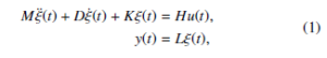
where the matrices M, D, K ∈ Rn×n are time-invariant, the input matrix H ∈ Rn×p describing the external access to the system and the output matrix L ∈ Rm×n represents the output of the measurement of the system. For M is an identity or invertible matrix, the system (1) is called a standard state-space system or can be converted into the standard state-space system. The system is n-dimensional, that contains the state vectors ξ(t) ∈ Rn, input (control) vectors u(t) ∈ Rp, and output vectors y(t) ∈ Rm. It is said to be continuoustime system as the input-output relations are established in the continuous-time interval [0,∞). The system (1) is specified as the Single-Input Single-Output (SISO) system for p = m = 1, and otherwise specified as the Multi-Input Multi-Output (MIMO) system, where p,m << n, i.e., the number of input and output of the system is much less than the number of states. If all the finite-eigenvalues of the matrix pencil of the system (1) lie in the left half-plane (C−), it is called asymptotically stable. This kind of dynamical systems emerge in several engineering disciplines such as automation & control systems, structural mechanics or multi-body dynamics, and electrical networks [1, 2, 3]. Applying the Laplace-transformation in the system (1), the transfer function that defines input-output mappings can be express as
![]()
Because of the arrangement of a large number of disparate devices and their complex structures, in the engineering applications most of the systems turn into very large-scale. The large-scale systems are infeasible for the simulation, controller design, and optimization within the computing tools for reasonable computational time and the memory allocation. To avoid the adversities, Model Order Reduction (MOR) can be applied to well-approximate the original models. So that, the aim of the automation & control systems can be fulfilled by reducing the work-load, feasible timemanagement and efficient use of system components. That is the system (1) needs to be replaced by the r-dimensional Reduced-Order Model (ROM) as
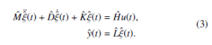
where Mˆ , Dˆ, Kˆ ∈ Rr×r, Hˆ ∈ Rr×p, Lˆ ∈ Rm×r and r n. The target is to minimize the value of r by the trial and error basis such that system (3) approximates the system (1) keeping the system properties invariant. The transfer-function corresponding to the ROM (3) is denoted by Gˆ and defined as
![]()
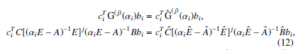
Some system oriented approximation requirements need to be fulfilled for the ROM (3), for instance the error norm ky(t) − yˆ(t)k or equivalently kG(.) − Gˆ(.)k needs to be optimized under appropriate norm estimation, for example H2, H∞ norms (see [4] and references therein).
Initially, the concept of interpolatory projection technique for MOR was developed in [5], and later updated in [6]. A modified approach was introduced in [7], in which the rational Krylov approach was implemented. In the MOR techniques for large-scale dynamical systems, Krylov based approaches can implicitly satisfy moment matching conditions avoiding the explicit computations to ignore the ill-conditioned simulations [8, 9]. A number of strategies have been flourished over the years for selecting the interpolation points and the tangential directions, which are the leading ingredients for finding the ROMs to get the best approximation of full models [10]. Nowadays selecting the suitable set of interpolation points is associated with the seeking of H2 optimality for MOR techniques [11]. The Iterative Rational Krylov Algorithm (IRKA) was developed that guarantees the H2 optimality of the investigation of interpolation points for MOR [12].
Definition-1: For the system (1), the H2 norm can be defined as
![]()
where G(jω)H is the harmonic conjugate of the frequency response G(jω) of the system and ω ∈ R is the frequency on the imaginary axis of the transfer function G(s) defined in (2). H2 norm is the most appropriate way to investigate the performance of the ROMs achieved by IRKA. Estimating the H2 norm by the improper integral (5) is impossible in practice.
Definition-2: The ROM (3) is said to be H2 optimal if Gˆ(s) is stable and minimize the error system under certain norm as
![]()
The details of the H2 norm of the error system defined in (6) will be discussed later in Section 4.
Usually in the present MOR approaches for the second-order systems (1) includes the conversion of second-order systems into equivalent first-order forms and imply some suitable MOR techniques to get the first-order ROMs, which is one of the most eyecatching drawbacks of the MOR technique as they are structure destroyer. Here we propose the MOR techniques for the secondorder system by applying the interpolatory techniques via IRKA, where the systems need not convert into the first-order form, that’s why the structure of the system remains invariant. Also, we estimate the minimized H2 error norm of the ROMs under a certain level of tolerance, by simulating the matrix equations governed from the error system.
2. IRKA for Model Order Reduction of First-Order Systems
To find the ROM of second-order systems through equivalent firstorder forms, there are a handful number of MOR techniques available implementing IRKA [13]. The interpolation-based techniques for the first-order generalized system has been reviewed in this section in brief. Let us consider the following first-order form
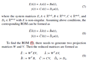
For the MIMO systems, interpolatory projection technique IRKA has been developed in [14], where the authors discussed that the interpolation points and the tangential directions need to be essentially updated until attain the H2 optimality. The distinct interpolation points, C and C are required to form right and left projector matrices W and V with the tangential directions bi ∈ Cm and ci ∈ Cp, respectively. Then these projector matrices need to be formed as
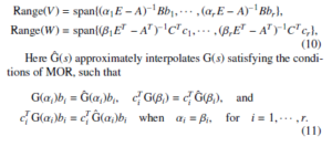
For a non-negative finite integer j, the following condition will be satisfied
where the j-th moment of G(.) is defined as C[(αiE −A)−1E]j(αiE −A)−1B, which evaluated at αi and represents the j-th derivative of G(.).
For the SISO systems, there need to consider the interpolation points but not the tangential directions. The complete procedures of IRKA for the SISO systems has been provided in [15].
The basis for the Krylov based MOR techniques require a adjustable interpolation points accomplishing the Petrov-Galerkin conditions [16]. The summary of the first-order IRKA procedures are provided in Algorithm 1 and Algorithm 2.
| Algorithm 1: IRKA for First-Order MIMO Systems. |
| Input :E, A, B,C, Da.
Output:Eˆ, Aˆ, Bˆ,Cˆ, Dˆ a := Da. 1 Consider the initial assumptions for the the interpolation points {αi}ri=1 and the tangential directions {bi}ri=1 & {ci}ri=1. h E − A)−1Bb1,··· ,(αrE − A)−1Bbri, 2 Construct V = (α1 W = (α1ET − AT )−1CT c1,··· ,(αrET − AT )−1CT cri. h 3 while (not converged) do 4 Find Eˆ = WT EV, Aˆ = WT AV, Bˆ = WT B, Cˆ = CV. 5 for i = 1,··· ,r. do 6Evaluate Azˆ i = λiEzˆ i and y∗i Aˆ = λiyi∗ Eˆ to find αi ← −λi, b∗i ← −y∗i Bˆ and c∗i ← Czˆ ∗i . 7 end for 8 Repeat Step-2. 9 i = i + 1; 10 end while 11 Find the reduced-order matrices by repeating Step-4. |
| Algorithm 2: IRKA for First-Order SISO Systems. |
| Input :E, A, B,C, Da.
Output:Eˆ, Aˆ, Bˆ, Cˆ, Dˆ a := Da. 1 Consider the initial assumptions for the the interpolation points {αi}ri=1. h −1B,··· ,(αrE − A)−1Bi, 2 Construct V = (α1E − A) W = (α1ET − AT )−1CT ,··· ,(αrET − AT )−1CT i. h 3 while (not converged) do 4 Find Eˆ = WT EV, Aˆ = WT AV, Bˆ = WT B, Cˆ = CV. 5 for i = 1,··· ,r. do 6Evaluate Azˆ i = λiEzˆ i and y∗i Aˆ = λiyi∗ Eˆ to find αi ← −λi. 7 end for 8 Repeat Step-2. 9 i = i + 1; 10 end while 11 Find the reduced-order matrices by repeating Step-4. |
3. IRKA for Structure-Preserving Model Order Reduction of Second-Order Systems
This section contributes the Structure-Preserving Model Order Reduction (SPMOR) of second-order system (1) via IRKA. One of the conversions of second-order system (1) into first-order form (7) is as follows
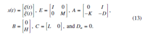
In the conventional techniques, to obtain an efficient ROMs of the second-order systems, at first, it is to convert into (13) essentially [17]. Then converted first-order form (7) can be implemented substantially and by applying Algorithm 1 or Algorithm 2 the equivalent first-order reduced order model (8) can be achieved.
Sometimes, that explicit formulation of (13) is prohibitive as the original model structure is destroyed and we cant return back to the original system. The structure preservation is essential for the large-scale secondorder systems to controller design, execute the computation, and optimization. SPMOR allows meaningful interpretation of the physical system and provides a more accurate approximation to the full model.
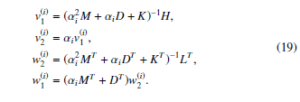
In the MIMO systems, to avoid the explicit conversion and derive the SPMOR approach, the i-th column of V and W utilizing the shifted linear systems need to be computed as
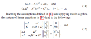
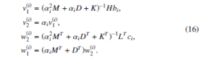
Albeit the matrices in (15) has higher dimension 2n, they are sparse and can be efficiently simulated by suitable direct or iterative solvers [18, 19]. After the elimination and simplification of the system of linear equations governed from (15) for v(1i), v2(i), w1(i) and w(2i), we have the followings
The concept of the formation (13) can be utilized in the system (7) and then by converting this to an equivalent sparse linear system, which ensures the structure preservation and rapid rate of convergence.
According to the techniques developed in [20], at each iteration, the first-order representation (13) will be considered and the Algorithm 1 will be applied to find desired set of interpolation points {αi}ri=1 efficiently. Also, Algorithm 1 updates the tangential directions {bi}ri=1 & {ci}ri=1 accordingly.
Due to the structure of system, we can split the desired projectors V and W as position and velocity levels [21]. We can partition the projectors V and W as
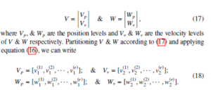
Again, for the SISO systems, to find the projectors V and W we need to consider the first-order representation (13) and apply the Algorithm 2 to find desired set of interpolation points {αi}ri=1 only. Then for the SISO systems, (16) turns into the followings
Since there are two sets of projectors as in (18), we will get two types of SPMOR for the system (1), position level and velocity level, respectively. We summarize the above ideas for computing SPMOR (3) in Algorithm 3 and Algorithm 4 for the second-order system (1).
| Algorithm 3: IRKA for Second-Order MIMO Systems. |
| Input :M, D, K, H, L.
Output:Mˆp, Dˆp, Kˆp, Hˆp, Lˆp, Mˆv, Dˆv, Kˆv, Hˆv, Lˆv. 1 Consider the initial assumptions for the the interpolation points {αi}ri=1 and the tangential directions {bi}ri=1 & {ci}ri=1. 2 Consider v(1i),v(2i),w(1i) and w(2i) are defined in (16) and construct Vp = [v(1)1 ,v(2)1 ,··· ,v(1r)] & Vv = [v2(1) ,v(2)2 ,··· ,v2(r)], Wp = [w(1)1 ,w(2)1 ,··· ,w(1r)] & Wv = [w2(1) ,w(2)2 ,··· ,w2(r)]. 3 while (not converged) do 4Find Mˆp = WpT MVp, Dˆp = WpT DVp, Kˆp = WpT KVp, Hˆp = WpT H, Lˆp = LVp. 5and Mˆv = WvT MVv, Dˆv = WvT DVv, Kˆv = WvT KVv, Hˆv = WvT H, Lˆv = LVv. 6Use the first-order representation (13) in Algorithm (1) to get Eˆ, Aˆ, Bˆ and Cˆ. 7Evaluate Azˆ i = λiEzˆ i and y∗i Aˆ = λiyi∗ Eˆ to find αi ← −λi, b∗i ← −y∗i Bˆ and c∗i ← Czˆ ∗i for all i = 1,··· ,r. 8Repeat Step-2. 9i = i + 1; 10 end while 11 Find the reduced matrices by repeating Step-4 and Step-5. |
| Algorithm 4: IRKA for Second-Order SISO Systems. |
| Input :M, D, K, H, L.
Output:Mˆp, Dˆp, Kˆp, Hˆp, Lˆp, Mˆv, Dˆv, Kˆv, Hˆv, Lˆv. 1 Consider the initial assumptions for the the interpolation points {αi}ri=1. (i) (i) (i) (i) 2 Consider v1 ,v2 ,w1 and w2 are defined in (19) and construct Vp = [v(1)1 ,v(2)1 ,··· ,v(1r)] & Vv = [v2(1) ,v(2)2 ,··· ,v2(r)], Wp = [w(1)1 ,w(2)1 ,··· ,w(1r)] & Wv = [w2(1) ,w(2)2 ,··· ,w2(r)]. 3 while (not converged) do 4Find Mˆp = WpT MVp, Dˆp = WpT DVp, Kˆp = WpT KVp, Hˆp = WpT H, Lˆp = LVp. 5and Mˆv = WvT MVv, Dˆv = WvT DVv, Kˆv = WvT KVv, Hˆv = WvT H, Lˆv = LVv. 6Use the first-order representation (13) in Algorithm (2) to get Eˆ, Aˆ, Bˆ and Cˆ. 7Evaluate Azˆ i = λiEzˆ i and y∗i Aˆ = λiyi∗ Eˆ to find αi ← −λi for all i = 1,··· ,r. 8Repeat Step-2. 9i = i + 1; 10 end while 11 Find the reduced matrices by repeating Step-4 and Step-5. |
4. Estimation of H2 error norm of the Reduced Order Model
The error system of the ROM (3) of the system (1) using the first-order representation (13) has the form
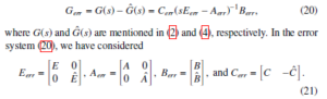
Here E, A, B and C are provided in the first-order representation (13) of the second-order system (1). Also, Eˆ, Aˆ, Bˆ and Cˆ are the reduced-order form of the first-order representation containing the reduced-order matrices defined in (3), which can be achieved by the Algorithm 3 for MIMO systems or Algorithm 4 for SISO systems.
Let us assume the controllability Gramian and observability Gramian for the error system (20) are Perr and Qerr, respectively, and they can be partitioned as
![]()
where P11, Q11 ∈ Rn×n, P22, Q22 ∈ Rr×r and P12, Q12 ∈ Rn×r. In terms of a Galerkin approach Gˆ(s) can be defined by considering the projectors V = P12P−221 and W , and the achieved ROM satisfies the desired first-order conditions of the optimal H2 norm condition with the property WT V = I [22].
The Gramians Perr and Qerr can be attained by simulating the following
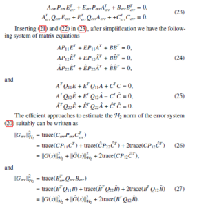
The H2 norm of the full model needs to be estimated once using the corresponding Gramians, and that is infeasible for a large-scale system by solving corresponding Lyapunov equations using the direct solvers. In this case, we can use the low-rank ADI based technique provided in Algorithm 1 of [23] or rational Krylov subspace method provided in Algorithm 2 of [24] to find the low-rank factors Zp and Zq of the Gramians P11 = ZpZTp and Q11 = ZqZqT defined in the first equations of (24) and (25), respectively. These approaches provide us feasible ways to find the H2 norm of the full model. Then, instead using the Gramians of the full model, we can use the low-rank Gramian factors in the first part of (26) and (27) as given below.
Since the Lyapunov equations defined by third equations in (24) and (25) corresponding to the ROMs are very small in size, they can be solved by any direct solver or MATLAB lyap command in every iterations to find the second part of (26) and (27), respectively. Moreover to find the third part of (26) and (27), we can solve the generalized Sylvester equations given in the second equations in (24) and (25), respectively, using the sparse-dense Sylvestor equation approach provided in Algorithm-4 of [25].
5. Numerical Results
The proposed techniques will be validated by applying them to the data generated from the real-world models given below. The computations will be carried out with the MATLAB R R2015a (8.5.0.197613) on a board with Intel RCoreTMi5 6200U CPU with 2.30 GHz clock speed and 16 GB RAM.
Example-1: [International Space Station Model (ISSM)] International Space Station Model is a part of modern aeronautics satisfying the second-order system defined in (1). This model is essential to control the system and maintain the varieties of operational modes at the international space station. The control of the system ensures the dynamic interaction within the components including adjustable structure alignments and clarification of the technical legitimacy of the flight.
The physical model of the international space station being assembled part by part. The modeling and control of the vibrations of the docking of an incoming spaceship is the prime concern under system constraints. Two types of ISSM exist for fulfilling the requirements of the space stations, namely the Russian service Module (1R) and the Extended Service Module [26]. In our work, we have taken the Russian service Module (12A) with state dimension n = 270 and the number of input-output is 3. The target model provides a sparse system derived from a complicated mechanical system.
Example-2 [Clamped Beam Model (CBM)] The Clamped Beam
Model is derived from micro-actuators, which is mainly a non-linear electrodynamic system satisfying a set of partial differential equations with the boundary conditions [27]. A usual micro-actuator combines two parallel conducting electrodes, one of which is movable and the rest is fixed. The movable electrode is formed as the clamped beam.
By the discretization approach Finite Element Method (FEM), the Clamped Beam Model has been derived as (1). For the Clamped Beam Model the state dimension n = 348 with single input-output. The force applied to the system at the movable end is taken as the input, whereas the resulting displacement is considered as the output.
Example-3 [Scalable Oscillator Model (SOM)] Scalable Oscillator Model is derived from a special class of mechanical systems consisting of three damping chains with all of the chains bonded to constant support by an extra damper at one end, whereas the other end of them bonded to a heavy and inflexible mass [28]. There are some amount of spring units that united the heavy mass. All of the three individual chains composed of n1 number of masses and unit springs with uniform stiffness. The masses m1, m2, m3 with the stiffness’s k1, k2, k3, respectively, are the model parameters for the desired model. For the bonding mass m0 is the mass with stiffness k0. Here ϑ is the viscosity of extra supporting damper and all of the individual oscillator chains.
The mathematical formulation of the Scalable Oscillator Model can be written in the form of the system (1) having the state dimension nξ = 3n1+1.
The matrix M = diag[m1In1,m2In1,m3In1,m0] represents the combination of the masses of the system with the stiffness K. The damping matrix D consists the stiffness of the oscillator chains as the elements in the block diagram form and the bonding terms in the last row and column at n1, 2n1 & 3n1 positions of the diagonals. The model used in the numerical computation of single input-output with state dimension n = 9001. For practical purposes, we have considered the following assumptions.
Example-4 [Butterfly Gyro Model (BGM)] For the applications of inertial navigation, vibrating micro-mechanical based Butterfly-Gyro is an essential engineering tool for its theoretical and practical contribution. The basic Butterfly-Gyro structure consists of a wafer stack of three layers with the body sensor in the middle. The model is named Butterfly-Gyro because of the existence of a pair of double wings attached with a common frame in the layout of the sensor [29].
The mathematical formulation employing the matrix equations has been governed from the physical model numerically using the multiphysics simulation software ANSYS7 and can be written as the system (1). The original derived model is a nξ = 17361-dimensional second-order system with single input but 12 outputs. To adjust the structure of our computation we have taken the transpose of the output matrix as the input matrix. Thus, in our work, the number of input-output is 12.
Above models discussed here are available in the web-page for the Oberwolfach Benchmark Collection[1] in detail.
Table 1 depicts the dimensions of the full models and their ROMs via IRKA based SPMOR achieved by the Algorithm 3 and Algorithm 4. Here the dimensions of the ROMs are taken appropriately such the ROMs approximate the corresponding full model sufficiently.
Table 1: Model examples and dimensions of full models and ROMs
Model type full model (n) ROM (r)
| ISSM | MIMO | 270 | 20 |
| CBM | SISO | 348 | 30 |
| SOM | SISO | 9001 | 50 |
| BGM | MIMO | 17361 | 70 |
The transfer functions of the full models and corresponding ROMs in the sense of position-level and velocity-level with the desired dimensions are compared in the Figure 1, Figure 2, Figure 3 and Figure 4 for the models discussed above. In each of the figures, the first sub-figures display the comparisons of the transfer functions of the full model and its ROMs considering both of the position-level and velocity-level, whereas the second and third sub-figures depict their absolute errors and relative errors, respectively.
Figure 1: Comparison of full model and ROM computed by Algorithm 3 (for MIMO
Figure 2: Comparison of full model and ROM computed by Algorithm 4 (for SISO system) of the ISSM
Figure 3: Comparison of full model and ROM computed by Algorithm 4 (for SISO
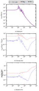
Figure 4: Comparison of full model and ROM computed by Algorithm 3 (for MIMO system) of the SOM
From the figures presented above, we have observed that the transfer functions of the full models and their ROMs of position-level and velocitylevel are nicely matched. For this reason, the absolute errors and the relative errors for all cases are sufficiently small. Therefore it can be said that the proposed IRKA based SPMOR technique for finding ROMs of both of the levels of the second-order systems is efficient and robust for the target models.
Speed-up of the frequency-responses of the target models represents in the Table 2. For the time-convenient comparison, we have measured the execution time of the frequency-responses for a single cycle of the full models and corresponding ROMs. The speed-up of the system execution indicates the feasibility of the time-allocation which is the fundamental requirement for the system automation and controller design. It has been noticed that the proposed technique is more efficient based on time for higher-dimensional models. Noted that the ROMs of position-level and velocity-level have the same execution time and for this, we have omitted to show them individually.
Table 2: Speed-up comparisons for ROMs
| Model | dimension | execution time (sec) | speed-up | |
| ISSM | full model
ROM |
270
20 |
5.67 × 10⁻⁴
2.04 × 10⁻⁴ |
2.78 |
| CBM | full model
ROM |
348
30 |
3.19 × 10⁻³
2.46 × 10⁻⁴ |
12.97 |
| SOM | full model
ROM |
9001
50 |
1.66 × 10⁻²
2.98 × 10⁻⁴ |
55.54 |
| BGM | full model
ROM |
17361
70 |
6.48 × 10⁻¹
1.07 × 10⁻³ |
609.13 |
In Table 3 the H2 error norms of the ROMs for the target models for both position-level and velocity-level have been illustrated. Here, to find the H2 norm of the full model we have used a low-rank ADI approach. It is observed that the H2 error norm for CBM is small enough and for ISSM it is better. For BGM, the H2 error norm is the best, whereas, for SOM, the H2 error norm is less satisfactory in comparison to other target models but still not intolerable. Thus, it is evident that the proposed techniques are capable to estimate the H2 optimal SPMOR for second-order systems with a few exceptions.
Table 3: H2 error norm of the ROMs
| Model | ROM | kG − GˆkH2 |
| ISSM | Position Velocity | 1.2 × 10⁻⁶
5.1 × 10⁻⁶ |
| CBM | Position Velocity | 1.1 × 10⁻³
3.6 × 10⁻³ |
| SOM | Position Velocity | 1.8 × 101
3.6 × 101 |
| BGM | Position Velocity | 6.6 × 10⁻¹²
7.8 × 10⁻¹² |
6. Conclusions
We have introduced the Structure-Preserving Model Order Reduction (SPMOR) techniques for second-order systems through the interpolatory projection-based method Iterative Rational Krylov Algorithm (IRKA). In those techniques, the second-order systems need not convert into the firstorder forms explicitly which are essential for preserving some important features of the systems. The SPMOR techniques enhance the rapid rate of convergence of the simulations and ensure the feasibility of further manipulations. We have derived the approaches to find the H2 error norm for the optimality condition of the Reduced-Order Models (ROM) achieved from the second-order systems, that confirm the fidelity of the proposed techniques. We have investigated the applicability and efficiency of the proposed techniques numerically using MATLAB simulation and applied them to some real-world models derived from engineering applications. From the numerical investigations, it is evident that the proposed techniques are efficient to find ROMs of the second-order systems, that can approximate the full models with reasonable absolute errors and relative errors. The speed-up of the target systems provided the testimony of the aptness of the proposed techniques in the automation and control systems. Finally, it can be concluded that proposed techniques provide ROMs of the second-order systems with the H2 optimal condition.
Acknowledgment
This work is funded by the Bangladesh Bureau of Educational Information and Statistics (BANBEIS) under a project bearing ID MS20191055. Also, the first author is affiliated to the University Grants Commission (UGC) of Bangladesh.
- R. Riaza, “Differential-Algebraic Systems. Analytical Aspects and Circuit Applications,” Singapore: World Scientific Publishing Co. Pte. Ltd., 2008.
- M. M. Uddin, J. Saak, B. Kranz, and P. Benner, “Computation of a compact state space model for an adaptive spindle head configuration with piezo ac- tuators using balanced truncation,” Production Engineering, 6, pp.577–586, 2012.
- M. M. Uddin, “Gramian-based model-order reduction of constrained structural dynamic systems,” IET Control Theory & Applications, 2018.
- S. Gugercin, A. C. Antoulas, and C. A. Beattie, “ 2 model reduction for large- scale dynamical systems,” SIAM J. Matrix Anal. Appl., 30(2), pp. 609–638, 2008.
- C. d. Villemagne and R. E. Skelton, “Model reductions using a projection formulation,” International Journal of Control, 46(6), pp.2141–2169, 1987.
- E. Grimme, “Krylov projection methods for model reduction,” Ph.D Thesis, University of Illinois at Urbana Champaign, May 1997. [Online]. Available: https://tel.archives-ouvertes.fr/tel-01711328
- A. Ruhe, “Rational Krylov algorithms for non-symmetric eigenvalue problems.ii. matrix pairs,” Linear algebra and its Applications, 197, pp.283–295, 1994.
- M. M. Uddin, “Computational methods for model reduction of large-scale sparse structured descriptor systems,” Ph.D. Thesis, Otto-von-Guericke- Universita¨t, Magdeburg, Germany, 2015. [Online]. Available: http:// nbn-resolving.de/urn:nbn:de:gbv:ma9:1-6535
- M. Uddin, “Numerical study on continuous-time algebraic Riccati equations arising from large-scale sparse descriptor systems,” Master’s thesis, Bangladesh University of Engineering and Technology, 2020.
- C. Lein, M. Beitelschmidt, and D. Bernstein, “Improvement of Krylov subspace reduced models by iterative mode-truncation,” IFAC-PapersOnLine, 48(1), pp. 178–183, 2015.
- G. Flagg, C. Beattie, and S. Gugercin, “Convergence of the iterative rational Krylov algorithm,” Systems & Control Letters, 61(6), pp.688–691, 2012.
- S. Gugercin, C. Beattie, and A. Antoulas, “Rational Krylov methods for optimal H2 model reduction,” submitted for publication, 2006.
- M. M. Uddin, “Computational Methods for Approximation of Large-scale Dynamical Systems,” Chapman and Hall/CRC, 2019.
- Y. Xu and T. Zeng, “Optimal 2 model reduction for large scale MIMO sys- tems via tangential interpolation,” International Journal of Numerical Analysis and Modeling, 8(1), pp. 174–188, 2011.
- K. Sinani, “Iterative rational Krylov algorithm for unstable dynamical systems and generalized co-prime factorizations,” Ph.D. dissertation, Virginia Tech, 2016.
- K. Carlberg, M. Barone, and H. Antil, “Galerkin v. least-squares Petrov– Galerkin projection in non-linear model reduction,” Journal of Computational Physics, 330, pp.693–734, 2017.
- P. Benner, P. Ku¨ rschner, and J. Saak, “An improved numerical method for balanced truncation for symmetric second order systems,” Mathematical and Computer Modelling of Dynamical Systems, 19(6), pp. 593–615, 2013.
- T.A. Davis, “Direct Methods for Sparse Linear Systems, Fundamentals of Algorithms,” Philadelphia, PA, USA: SIAM, 2006.
- Y. Saad, “Iterative Methods for Sparse Linear Systems,” Philadelphia, PA, USA: SIAM, 2003.
- S. A. Wyatt, “Issues in interpolatory model reduction: Inexact solves, second- order systems and DAEs,” Ph.D. dissertation, Virginia Tech, 2012.
- P. Benner and J. Saak, “Efficient balancing-based mor for large-scale second- order systems,” Mathematical and Computer Modelling of Dynamical Systems, 17(2), pp. 123–143, 2011.
- D. A. Wilson, “Optimum solution of model-reduction problem,” in Proceedings of the Institution of Electrical Engineers, 117(6), pp.1161–1165, 1970.
- S. Hasan, A. M. Fony, and M. M. Uddin, “Reduced model based feedback stabilization of large-scale sparse power system model,” in International Con- ference on Electrical, Computer and Communication Engineering (ECCE),
IEEE, 2019, pp.1–6. - M. M. Uddin, M. S. Hossain, and M. F. Uddin, “Rational Krylov subspace method (RKSM) for solving the lyapunov equations of index-1 descriptor sys- tems and application to balancing based model reduction,” in 9th International Conference on Electrical and Computer Engineering (ICECE), IEEE, 2016, pp.451–454.
- P. Benner, M. Ko¨ hler, and J. Saak, “Sparse-dense Sylvester equations in H2- model order reduction,” 2011.
- S. Gugercin, A. Antoulas, and N. Bedrossian, “Approximation of the interna- tional space station 1R and 12A models,” in Proceedings of the 40th IEEE Conference on Decision and Control (Cat. No. 01CH37228), 2, IEEE, 2001, pp. 1515–1516.
- A. C. Antoulas, D. C. Sorensen, and S. Gugercin, “A survey of model reduction methods for large-scale systems,” Contemp. Math., 280, pp.193–219, 2001.
- N. Truhar and K. Veselic´, “An efficient method for estimating the optimal dampers’ viscosity for linear vibrating systems using Lyapunov equation,” SIAM J. Matrix Anal. Appl., 31(1), pp.18–39, 2009.
- J. Lienemann, D. Billger, E. B. Rudnyi, A. Greiner, and J. G. Korvink, “MEMS compact modeling meets model order reduction: Examples of the application of Arnoldi methods to microsystem devices,” in the technical proceedings of the 2004 nanotechnology conference and trade show, Nanotech, 4, 2004.
No related articles were found.