
Bathtub-Shape Failure Rate Life Time Model in a New Version with the use of Bayesian Prediction Bounds for the Presence of Outliers
Volume 5, Issue 4, Page No 710-714, 2020
Author’s Name: Ayed Rheal A. Alanzia)
View Affiliations
Mathematics Department, Faculty of Science and Human Studies of Hotat Sudair, Majmaah University, Majmaah 11952, Saudi Arabia
a)Author to whom correspondence should be addressed. E-mail: a.alanzi@mu.edu.sa
Adv. Sci. Technol. Eng. Syst. J. 5(4), 710-714 (2020); ![]() DOI: 10.25046/aj050484
DOI: 10.25046/aj050484
Keywords: Outliers, Censored Samples, Bayesian Prediction, Bivariate Prior, Bathtub-Shaped Model, Density Function

Export Citations
The present article explains obtaining of the Bayesian prediction bounds at the maximum and minimum rate taking into account the results of future observation from a new version of a bathtub-shape failure rate distribution of life time type in the presence of outliers. The Type-II censored sample serves as a basis for the intervals of the prediction with the numerical examples as illustrations of the studied procedure.
Received: 06 May 2020, Accepted: 24 July 2020, Published Online: 28 August 2020
1. Introduction
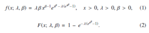
Researchers study numerous statistical problems with the requirement to apply the same distribution on the basis of the previously obtained data to predict the future data. Previous analysis of various practical applications required to satisfy the mentioned needs have been conducted in the studies of [1]-[3] with the most prominent suggestions and analysis done in the study of [4]. The latter is devoted to analysis of the bathtub-shaped distribution of life-time type, taking into account the function of increasing failure rate or two parameters. Provided that the distribution is shown with λ and β as the available two parameters by Chen, it is possible to present the functions of probability density and cumulative distribution in the equations as follows:
The calculations of [5] presented Bayesian estimations on the basis of bathtub-shaped life time distribution of two parameters with the use of record values. The study of [6] is devoted to obtaining bounds of Bayesian prediction for a life time distribution with the function of bathtub-shaped failure rate on the basis of two parameters. Based on censored data, [7] suggested a two-parameter Lifetime Distribution with Bathtub Shaped Hazard. Consequently, derivation of Bayesian prediction bounds was done by [8] for a new version of bathtub shape failure rate life time model of doubly typeII censored samples. Their research was of crucial importance, taking into consideration the functions of life time distribution founded upon the Bayesian intervals for prediction [9]. E-Bayesian estimation of Chen distribution based on type-I censoring scheme has also investigated [10].
Application of prediction techniques with two samples was done with the use of the parameters obtained previously for a single problem of statistical significance. The key problem of the outlier presence was identified with several approximation approaches combined, and it produces an impact on the estimations of previous density with implementation of unknown parameters. Illustration of the significance of the presented problem from a statistical perspective is done with numerical estimation and gamma conjugate joint prior and prior cases. The present research studies Bayesian prediction intervals from the Chen (λ,β) model (1) for future observations under two plans of sampling: x(1), x(2), · · · , x(n) is an ordered random sample from model (2) (size n) where x(r), x(r+1), · · · , x(n), the (n−r) are the sample ordered observations of the largest size. Statistical analysis applies the ordered observations which remained, i.e., x = (x(1), · · · , x(r)). It is evident that the sampling has its special cases like a complete ordered sample (r = n).
In the first case, the observed sample is presented as follows:
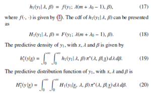
x(1) < · · · < x(r) is Type II censored sample with r < n. An unobserved sample is presented with x(r+1) < x(r+2) < · · · x(n) as remaining values. The observed sample is used for the study of the remaining n − r values.
In the second case, the previously mentioned Type II of sample is represented in the same way as x(1) < · · · < x(r). The future unobserved sample is shown as z1 < z2 < · · · < zm from the same population. The key aim for the selected configurations of sampling is identification of the prediction intervals with the applied previous observations for specification of the future observations.
Derivation of a random sample x(1) < x(2) < · · · < x(n) is done with the probabilities specified in (1) and (2) from the a population. In addition, the life test uses the assigned x1, x2, · · · , xn Recording of the failure times is done from the timeframe of rth failure with r < n. The following likelihood function estimate is used for the Type-II censored data with the mentioned observations, taking into account:
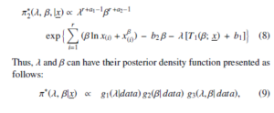
 According to the suggestion of [11], the function presented in (6) and (7) can be used to identify the bathtub-shaped distribution with the help of two parameters. Summarization of the function of joint posterior density that λ and β parameters have can be done as follows with the help of the joint prior density function presented correspondingly in (14) and (19) as well as the likelihood function:
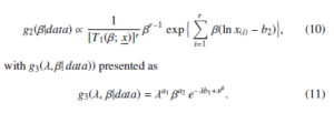
with g1(λ|β,data) as a gamma density with the constraints of the r shape and T1(β; x) scale, while g2(β|data) can be viewed as a function of proper density estimated as follows:
Hence, the following equation presents the Bayesian estimation of λ and β in any function, for instance g(λ, β) under the function of squared error loss:
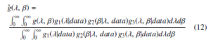
As for the equation (21), conversion is evidently impossible with the output of a simple closed form; that implies that estimations of the Bayesian predications for the inputs of λ and β specified before are impossible in this form as well. Consequently, it can be suggested to follow the recommendation in [12] and use the approach of importance sampling technique for approximation of (21) with reference to the restriction of a simple closed form.
1.1 Importance sampling technique
The methodology of an importance sampling technique is applied for computing and validating the Bayes estimates on λ and β as well as g(λ, β) and other constructed relevant functions. Algorithm presents the function of posterior density with the peculiar features of the process of approximation.
Algorithm 1: Sampling Technique Algorithm
Step 1: Estimation of β on the basis of g1(β|data).
Step 2: Estimation of λ on the basis g2(λ|β,data).
Step 3: Repetition of the described stages following the principle of consecutiveness aimed at generating (λ1, β1), (λ2, β2), · · · , (λM, βM)
The following equation presents the process of approximation using the restrictions of Bayesian estimates for g(λ, β) and squared error loss control in the framework of the procedure of importance sampling:
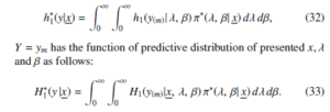
2. Bayesian prediction under the condition of the presence of outliers
This part of research is devoted to predicting of future outputs of the studies in the presence of outliers. All the formal definitions used in this section are the same as in (1) and x1, x2, · · · , xn is used as a random sample formed for the given function of the population density from Chen (λ,β). Furthermore, y1, y2, · · · , ym is referred to as independent unobserved sample generated from the same data points, further denoted as a future sample. Furthermore, we probe the limits of Bayesian prediction for sth in the framework of the future estimates that ys, s = 1, 2, · · · , m has under the conditions of using single outliers. The following equation presents the ys density function under the mentioned conditions for θ:
The functions of density and cumulative distribution are presented as f = f(y| θ) and F = F(y|θ) for any ys provided that they cannot be referred as outliers with outliers as f∗ = f∗(y|θ) and F∗ = F∗(y|θ) [13]. The change of λ parameter by λλo or λ depending on the classification of the outliers allows obtaining the f∗ and F∗ functions for the Chen (λ,β) model.
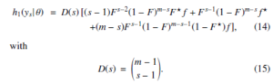
3. Predicting the minimum
It is possible to present distribution in the minimum in m-sized future sample with the single outlier of type λλo given by using s as 1 in (14) as follows:
![]()
It is possible to obtain the density function of Y1 in the case of Chen (λ,β) in the presence of a single type λλ0 outlier via substitution of (1) for f and (2) for F correspondingly in (16). f∗ and F∗ have values given by (1) and (2) further after λ is replaced by λλ0. Simplification of this density function is done in the following form:
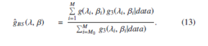
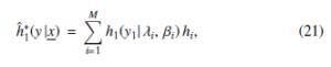
It can be assumed that {(λi, βi); i = 1, 2, · · · , M} should be viewed as MCMC samples obtained from π∗(λ, β| x). The equation for corresponding estimation parameters that consistency of h , λ, β) and H∗(y1|x, λ, β) has is as follows:
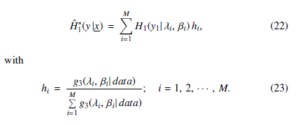
All the mentioned equations serve as the basis for the a
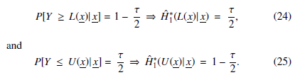
(1 − τ)100% Bayesian estimation for Y1 , which implies having P[L(x) ≤ Y1 ≤ U(x)] = 1 − τ, with L(x) as the highest and limit for y1 and U(x) as the lowest limit for y1. On the basis of the prior estimates for (22), 1 − and , we can claim that
Computing of the prediction bounds of y1 is done on the basis of the (24) and (25) equations.
4. Predicting the maximum
Obtaining of distribution of the maximum in a m-sized sample with the presence of a single outlier is done via using s = m in (14). The equation for Ym density function for a provided θ in the presence of a single outlier is as follows:
![]()
It is possible to obtain the density function of Ym in the case of Chen(λ, λ) in the presence of a single type λλ0 outlier via substitution of (1)for f and (2) for F correspondingly in (26). f∗ and F∗ have values given by (1) and (2) further after λ is replaced by λλ0. Simplification of this density function is done in the following form:
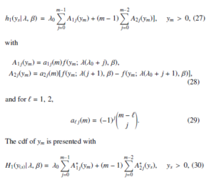
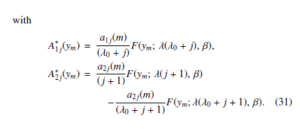
Table 1: Bayesian prediction intervals (95%) for y1 and y10 in the presence of type λλ0 single outlier, r = 20,n = 30. Note: PP is Point Predictor, L is Lower bound, U is Upper bound, and CP is Coverage Percentage
| λ0 | Observations | y1 | y10 |
| 1 | PP | 0.219311 | 1.03915 |
| L | 0.037503 | 0.773876 | |
| U | 0.470244 | 1.30324 | |
| Length | 0.432741 | 0.529363 | |
| C P | 95.45 % | 94.85 % | |
| 2 | PP | 0.209173 | 1.02768 |
| L | 0.035691 | 0.757975 | |
| U | 0.449826 | 1.29739 | |
| Length | 0.414135 | 0.539419 | |
| CP | 94.6 % | 95.16 % | |
| 3 | PP | 0.200296 | 1.02638 |
| L | 0.034113 | 0.085392 | |
| U | 0.431811 | 1.19415 | |
| Length | 0.397698 | 1.10876 | |
| CP | 93.77% | 88.02% | |
| 4 | PP | 0.192439 | 1.02614 |
| L | 0.032723 | 0.751878 | |
| U | 0.415762 | 1.29738 | |
| Length | 0.383039 | 0.545498 | |
| CP | 92.59% | 95.36% | |
| 5 | PP | 0.185422 | 1.02609 |
| L | 0.031487 | 0.751374 | |
| U | 0.401347 | 1.29738 | |
| Length | 0.36986 | 0.546003 | |
| CP | 91.54% | 95.4% |
Obtaining the h , λ, β) and H∗(y(m)|x, λ, β) as simulation consistent estimators can be done in the following manner assuming that (λi,βi);i = 1,2, · · · , M can be viewed as MCMC samples generated from π∗(λ, β| x):
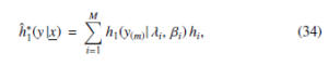
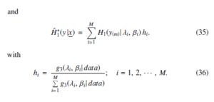
Table 2: Bayesian prediction intervals (95%) for y1 and y10 in the presence of type λλ0 single outlier, r = 25,n = 30. Note: PP is Point Predictor, L is Lower bound, U is Upper bound, and CP is Coverage Percentage
| λ0 | Observations | y1 | y10 |
| 1 | PP | 0.225826 | 1.04406 |
| L | 0.039754 | 0.782087 | |
| U | 0.479422 | 1.30373 | |
| Length | 0.439668 | 0.521645 | |
| CP | 95.4 % | 94.46% | |
| 2 | PP | 0.215545 | 1.03274 |
| L | 0.037862 | 0.766312 | |
| U | 0.458946 | 1.298 | |
| Length | 0.421084 | 0.531691 | |
| CP | 94.75% | 94.91% | |
| 3 | PP | 0.206536 | 1.03146 |
| L | 0.036213 | 0.761754 | |
| U | 0.440865 | 1.29799 | |
| Length | 0.404652 | 0.536232 | |
| CP | 94.01 % | 95.06 % | |
| 4 | PP | 0.198558 | 1.03123 |
| L | 0.034759 | 0.760261 | |
| U | 0.424745 | 1.29799 | |
| Length | 0.389986 | 0.537724 | |
| CP | 93.18 % | 95.1% | |
| 5 | PP | 0.191427 | 1.03117 |
| L | 0.033465 | 0.759761 | |
| U | 0.410255 | 1.29799 | |
| Length | 0.37679 | 0.538224 | |
| CP | 92.12 % | 95.11 % |
A 100% Bayesian prediction interval (1 − τ) for Ym can be presented as P[L(x) ≤ Ym ≤ U(x)] = 1 − τ,, with L(x) as the lower bound for ym and U(x) as the upper bound for ym. Thus equating (35) 1 − and , it is possible to get the following equations:
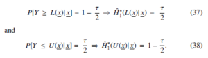
Solutions to (37) and (38) as nonlinear equations are found with the use of an iterative method aimed at evaluating the Bayesian prediction and obtaining its lower and upper bounds for the future sample ym at its maximum point.
Example. I can use the previous (6) density equation to generate λ = 1.41617 with the provided previous parameters a1 = 2.2 and b1 = 1.8 and then we use the previous (7) density equation to generate β = 1.91297 for the previous parameters a2 = 3.2 and b2 = 1.5. Chen distribution (λ = 1.41617, β =,1.91297) with r in its deferent value is used to generate a random sample of size n = 30. Let us consider a case with one more sample of size m = 10 in the presence of type λλ0 single outlier. Our aim is to obtain the percentage of 95% as prediction bounds for Y1 and Y10 for the provided value of λ0 as minimum and maximum that the future sample has. Table 1, Table 2, and Table 3 present the mentioned bounds with λ0 in corresponding values.
Table 3: Bayesian prediction intervals (95%) for y1 and y10 in the presence of type λλ0 single outlier, r = n = 30. Note: PP is Point Predictor, L is Lower bound, U is Upper bound, and CP is Coverage Percentage
| λ0 | Observations | y1 | y10 |
| 1 | PP | 0.225842 | 1.04428 |
| L | 0.039745 | 0.782243 | |
| U | 0.479499 | 1.304 | |
| Length | 0.439754 | 0.521755 | |
| CP | 95.4% | 94.44% | |
| 2 | PP | 0.21556 | 1.03295 |
| L | 0.037853 | 0.133706 | |
| U | 0.459018 | 1.19737 | |
| Length | 0.421165 | 1.06367 | |
| CP | 94.75% | 88.47% | |
| 3 | PP | 0.206549 | 1.03168 |
| L | 0.036204 | 0.761905 | |
| U | 0.440932 | 1.29825 | |
| Length | 0.404728 | 0.536345 | |
| CP | 94.02 % | 95.07% | |
| 4 | PP | 0.198569 | 1.03144 |
| L | 0.03475 | 0.760412 | |
| U | 0.424807 | 1.29825 | |
| Length | 0.390057 | 0.537837 | |
| CP | 93.18% | 95.1% | |
| 5 | PP | 0.191436 | 1.03138 |
| L | 0.033457 | 0.035391 | |
| U | 0.410314 | 1.09987 | |
| Length | 0.376857 | 1.06448 | |
| CP | 92.12% | 68.35% |
5. Conclusion
The present study analyzes a single type λλ0 outlier as the multiple outliers are more complicated. In case of no outliers in the homogeneous case,future observations can obtain Bayesian prediction bounds at the minimum and maximum level via assigning λ0 = 1 for the (22) and (35) equations. Table 1 demonstrates that future observations have their limits dependent on λ value.
Conflict of Interest
The authors declare no conflict of interest.
Acknowledgment
The author thanks to the Deanship of Scientific Research at Majmaah University for support and encouragement.
- I. R. Dunsmor, “The Bayesian predictive distribution in life testing models.” Technometrics, 16(3), 455-460, 1974. https://doi.org/10.1080/00401706.1974.10489216
- A. Aitchison, and I.R. Dunsmore, “Statistical Prediction Analysis”, Cambridge University Press, 1975.
- S. Geisser, Predictive inference 55 CRC press, 1993.
- Z. Chen, “A new two-parameter lifetime distribution with bathtub shape or increasing failure rate function”. Statistics and Probability Letters 49, 155-162, 2000. https://doi.org/10.1016/S0167-7152(00)00044-4
- M.A. Selim, “Bayesian Estimations from the Two-Parameter Bathtub- Shaped Lifetime Distribution Based on Record Values”. Pakistan Journal of Statistics and Operation Research 8(2):155-165, 2012. https://doi.org/10.18187/pjsor.v8i2.328
- S. F. Niazi and A. M. Abd-Elrahman “Bayesian prediction bounds for a two- parameter lifetime distribution with bathtub-shaped failure rate function”. SYL- WAN 159(6), 34-50, (2015).
- A. M. Sarhan, & J. Apaloo, “Inferences for a two-parameter lifetime distribu- tion with bathtub shaped hazard based on censored data”. International Journal of Statistics and Probability, 4(4), 77-92, 2015.
- S. F. Niazi and A. M. Abd-Elrahman, “Bayesian prediction bounds of doubly type-ii censored samples for a new bathtub shape failure rate life time model”. Journal of Applied Mathematics and Statistical Sciences 1(2), 21-30, 2016.
- A. R. Alanzi and S. F. Niazi, “Bayesian Prediction Intervals For A New Bathtub Shape Failure Rate Lifetime Model In The Presence Of Outliers”. Advances and Applications in Statistics, 63, Pages 1-22, 2020.
- A. Algarni, A. M. Almarashi, H. Okasha, & H. K. T. Ng, “E-Bayesian Estima- tion of Chen Distribution Based on Type-I Censoring Scheme”. Entropy, 22(6), 636, 2020. https://doi.org/10.3390/e22060636
- A. M. Sarhan, D. C. Hamliton, and B. Smith, “Parameter estimation for a twoparameter bathtub-shaped lifetime distribution” Applied Mathematical Modelling, (36), 5380-5392, 2012. https://doi.org/10.1016/j.apm.2011.12.054
- M. H. Chen, & Q. M. Shao, “Monte Carlo estimation of Bayesian credible and HPD intervals”. Journal of Computational and Graphical Statistics, 8(1), 69-92, 1999. https://doi.org/10.1080/10618600.1999.10474802
- N. Balakrishnan, & R. S. Ambagaspitiya, “Relationships among moments of order statistics in samples from two related outlier models and some applica- tions”. Communications in Statistics-Theory and Methods, 17(7), 2327-2341, 1988. https://doi.org/10.1080/03610928808829749