1. Introduction

This paper is an extension of work originally presented in conference CSIT-2019 [1].

The term “logical approach to solving Artificial Intelligence (AI) problems” is usually understood as data notation in the form of a binary string that defines the values of some object properties under study. In this case, if the object is represented as a set of its elements that have some properties and are connected by given relations, then when describing it as a binary string, firstly, the structure of the object itself is lost, and secondly, you have to store a large number of “unnecessary” information that the element a_j does not have the properties p_i1,…, p_ik , that the elements a_j1,a_j2 are not in the relations q_i1,…,q_il , etc.

Consider objects composed of smaller elements with preassigned properties, and some smaller object having preassigned relations. In such a case predicate formulas are an adequate description language.

The use of predicate calculus and automatic proof of a theorem for AI problems solving was offered by many authors [2]-[4] in the 70-th years of the XX century. At the same time the notion of NP-completeness was introduced and began to be actively used by the scientific community [5].

In 2003 the use of predicate calculus and automatic proof of a theorem for AI problems solving (without complexity bounds) was described in [6].

In particular, in that book it is shown that if a binary string simulates a description of an economic problem in which interaction agents have given properties and are in given relations then the notation length of such a string is exponential of the length of the description of the same problem input data by setting properties of these agents and relations between them, i.e. in fact, using the language of predicate calculus.

In 2007 the author of this paper has proved NP-completeness of recognition problems described in the terms of predicate formulas and upper bounds of number of steps for two solving algorithms [7]. When such problems are solved by an exhaustive search algorithm, their computational complexity coincides with the length of their input data encoding using a binary string [6].

A hierarchical level description of classes was suggested in [8] to decrease the computational complexity of these problems. Formulas which are isomorphic to “frequently appeared” sub-formulas of “small complexity” are extracted from class descriptions in order to construct such a level description. This allows to decompose the main problem into a series of similar problems with input data with the smaller length. An instrument for this extraction is partial deduction of a predicate formula [9],[10].

Later, the author noticed that the level description is actually a recognition network, which, after training (having exponential computational complexity), can quickly solve the recognition problem.

The concept of “network” is increasingly used both in theoretical and in practical research, particularly, when solving pattern recognition problems. Research and practical applications of neural networks [11],[12], Bayesian networks [13]-[15], technical networks [16] are widespread. The inputs of such networks are usually signals characterizing the properties of the studied objects or processes, and expressed, as a rule, by numerical characteristics, which can be encoded by binary strings. The processing of binary strings in the most cases is carried out in linear or polynomial (usually quadratic) number of steps under the length of these strings. A convenient model for processing such strings is propositional logic (Boolean functions).

As noted above, the use of binary strings in the recognition of complex structured objects has disadvantages. To recognize such objects, the author offered the notion of a logic-predicate network using level description of classes [17]. Such a network contains two blocks: a training block and a recognition block. The training block run is based on the extraction from a class of objects description such fragments, which are inherent in many objects of the class. Recognition block run is reduced to the sequential solution of problems of the same type with a smaller length of the input data.

The disadvantage of such a recognition network is that it is able to recognize only objects that differ from those included in the training set (TS) by renaming the elements of the object (objects with isomorphic descriptions). But such a network can be retrained by adding unrecognized objects to the TS. This was the reason for modification of the logic-predicate network permitting to recognize objects, that not coincide but only similar to the objects from a training set. Such a modification was offered in [1, 18]. The degree of coincidence for description of an object part and the formula, satisfiability of which is checking in the cell, is calculated. Such a fuzzy network allows not only quickly enough to recognize objects isomorphic to those represented in the TS, but also to calculate the degree of coincidence that a “new” object belongs to one or another class. If necessary, it can be retrained using such a “new” object.

The structure of the paper is as follows. Section 2 “Logic-predicate approach to AI problems” contains 2 subsections: “Problem Setting” and “Important Definitions”. This section describes the results previously obtained by the author and defines the terminology previously introduced by the author, which are necessary for understanding the further presentation.

Section 3 “Level description” presents the basic idea of constructing a level description of classes. It contains two sub-sections “Construction of a level description of classes” and “The use of level description of a class”. They give algorithms for constructing a level description of classes and the use of such a description for object recognition. These algorithms are further used in constructing the logic-predicate network. It is shown that the computational complexity of an object recognition decreases while using a level description of a class.

Section 4 “Logic-predicate network” describes the structure of such a network.

Section 5 “Example of logic-predicate network” describes an example illustrating the formation of a network, recognizing of an object with the use of a network, and its retraining. It consists of 4 sub-sections “Training Block Run: Extraction of Sub-Formulas”,

“Training Block Run: Forming a Level Description”, “Recognition Block Run” and “Retraining the Network”.

Section 6 “Fuzzy recognition by a logic-predicate network” describes the changes that need to be made to the logic-predicate network in order to recognize objects that are not isomorphic to those presented in the TS. A description of the contents of a fuzzy network cell is given. A cell of this type replaces each cell in the logic-predicate network in which the logical sequence of the target formula from the description of an object is checked. In this case, the degree of coincidence is calculated that the fragment being tested partially (and to what extent) satisfies the target formula.

Section 7 “Model example of fuzzy recognition” presents an example of fuzzy recognition of a “new” object.

In comparison with [1], the setting of problems that can be solved in the framework of logic-predicate approach are described in the presented paper in more details. A justification for the introduction of a level description is given. Algorithms for a level description construction and a level description use are described. Scheme 1 of a common up to the names of arguments sub-formulas extraction is added. A section 5 has been added with an example of constructing and modifying a logic-predicate network. It describes in details how a network is formed by the training set, a new object is recognized, and the network is rebuilt. The scheme of a fuzzy logic-predicate network cell is presented. An example of fuzzy recognition is described in more details.

2. Logic-Predicate Approach to AI Problems

A detailed presentation of the logic-predicate approach to solving AI problems is available in [19]. In this paper only a general setting of problems and main methods for their solving are formulated.

2.1          Problem Setting

As it was mentioned in the Introduction, if an object to be recognized is a complex structured one, then predicate formulas are a convenient language for its description and recognition. Let an investigated object ω be represented as a set of its elements ω = {ω₁,…,ω_t} and be characterized by predicates p₁,…, p_n which define some properties of its elements or relations between them. The description S(ω₁,…,ω_t) of the object ω is a set of all constant literals (atomic formulas or their negations) with predicates p₁,…, p_n which are valid on ω.

Let the set of all investigated objects Ω be is divided into classes Ω₁,…,Ω_K such that _k. Logical description of the class Ω_k is such a formula A_k(x)^[1] that if the formula A_k(ω) is true then ω ∈ Ω_k. The class description may be represented as a disjunction of elementary conjunctions of atomic formulas.

Many AI problems may be formulated as follows with the use of such descriptions.

Identification problem. To pick out all parts of the object ω which belong to the class Ω_k

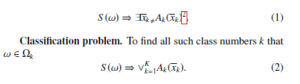
Analysis problem. To find and classify all parts τ of the object ω which may be classified

In fact, instead of the quantifier ∃ (whether exists) a symbol ?

(for what) must be written. But if one uses a constructive method of its proof (an exhaustive search algorithm or logical methods such as derivation in a sequential predicate calculus or resolution method for predicate calculus) then not only existence of such arguments would be proved but the values of them would be found.

It was proved that the problems (1) and (3) are NP-complete [7] and the problem (2) is GI-complete [20], i.e. it is polynomially equivalent to the “open” problem of Graph Isomorphism, for which it is not proved its NP-completeness and a polynomial in time algorithm is not found.

As the formulas A_k(x_k) may be represented as a disjunction of elementary conjunctions of atomic formulas, the checking of each of the problems (1), (2) and (3) may be reduced to sequential checking of the formula

where A(x) is an elementary conjunction. Note that in the case of the problem (2) the number of variables in x equals to the number of constants in ω.

The formula (4) may be checked, for example, by an exhaustive algorithm and an algorithm based on the derivation in sequential calculus or on the use of resolution method.

The upper bound of number of steps for an exhaustive algorithm is O(t^m)^[3], where t is the number of elements in ω, m is the number of variables in A(x) [7]. This upper bound coincides with the upper bound of a binary string simulating input data in the form of S(ω) and A(x).

The upper bound of the number of steps for a logical algorithm is O(s^a) where s is the maximal number of atomic formulas in S(ω) with the same predicate symbol having occurrences in A(x), a is the number of atomic formulas in the elementary conjunction A(x) [21].

Obviously, these estimates depend exponentially on the parameters of the formula A(x). That’s why it will be useful to break the solution of the problem into a series of sub-problems of the type (4) with a shorter right-hand side.

2.2        Important Definitions

The objects and notions satisfying the following definitions will be used later in the text.

Definition 1: Elementary conjunctions P(a₁,…,a_m) and Q(b₁,…,b_m) are called isomorphic P(a₁,…,a_m) ∼ Q(b₁,…,b_m),

if there are an elementary conjunction R(x₁,…, x_m) and substitutions of arguments a_i1,…,a_im and b_j1,…,b_jm instead of the variables x₁,…, x_m such that the results of these substitutions R(a_i1,…,a_im ) and R(b_j1,…,b_jm ) coincide with formulas P(a₁,…,a_m) and Q(b₁,…,b_m), respectively, up to the order of literals.

The substitutions (a_i1 → x₁,…,a_im → x_m) and (b_j1 → x₁,…,b_jm → x_m) are called unifies of R(x₁,…, x_m) with P(a₁,…,a_m) and Q(b₁,…,b_m) and are denoted as λ_R,P and λ_R,Q, respectively. [1], [20]

Note that concept of isomorphism of elementary conjunctions of atomic predicate formulas differs from the concept of equivalence of these formulas, because they can have significantly different arguments. In fact, for isomorphic formulas there are permutations of their arguments such that they define the same relationship between their arguments.

Definition 2: Elementary conjunction C(x₁,…, x_n) is called a common up to the names of arguments sub-formula of two elementary conjunctions A(a₁,…,a_m) and B(b₁,…,b_k) if it is isomorphic to some sub-formulas A⁰(a⁰₁,…,a⁰_n) and B⁰(b⁰₁,…,b⁰_n) of A(a₁,…,a_m) and B(b₁,…,b_k), respectively. The unifiers of C(x₁,…, x_n) with A⁰(a⁰₁,…,a⁰_n) and B⁰(b⁰₁,…,b⁰_n) will be denoted as λ_C,A and λ_C,B, respectively [19].

For example, let A(x,y,z) = p₁(x) & p₁(y) & p₁(z) & p₂(x,y) & p₃(x,z),

B(x,y,z) = p₁(x) & p₁(y) & p₁(z) & p₂(x,z) & p₃(x,z).

The formula P(u,v) = p₁(u) & p₁(v) & p₂(u,v) is their common up to the names of variables sub-formula with the unifiers λ_P,A = (x → u,y → v) and λ_P,B = (x → u,z → v) because P(x,y) = p₁(x)&p₁(y)&p₂(x,y) is a sub-formula of A(x,y,z) and P(x,z) = p₁(x)&p₁(z)&p₂(x,z) is a sub-formula of B(x,y,z).

Definition 3: Elementary conjunction C(x₁,…, x_n) is called a maximal common up to the names of arguments sub-formula of two elementary conjunctions A(a₁,…,a_m) and B(b₁,…,b_k) if it is their common up to the names of arguments sub-formula and after adding any literal to it, it ceases to be one [19].

For further presentation, the concept of partial sequence [9] is important.

The problem of checking if the formula A(x) or some its subformula A⁰(y) is a consequence of the set of formulas S(ω) is under consideration in [9]. Here the list of arguments y⁰ is a sub-list of the list of arguments y.

Definition 4: Let A(x) and B(y) be elementary conjunctions.

A(x) ⇒ ∃y_, B(y) is not valid but for some sub-formula B⁰(y⁰) of B(y) the sequence A            ) is true, we will say that B(y) is a partial sequence from A(x) and denote this by A(x) ⇒_P ∃y_, B(y) [1].

A constructive algorithm for a proof of partial sequence is in [22]. While using a constructive algorithm to prove A(x) ⇒_P ∃y_, B(y) we can find the maximal sub-formula B⁰(y⁰) such that A(x) ⇒ ∃y⁰_, B⁰(y⁰) and such values x⁰ (x⁰ is a permutation of a sub-string of x) for y⁰ that B⁰(x⁰) is a sub-formula of A(x). It means that we find a maximal common up to the names of arguments sub-formula B⁰(y⁰) of two elementary conjunctions A(x) and B(y) and its unifier with B⁰(x⁰) (a sub-formula of A(x)).

Further, for fuzzy recognition of an object we need an extension of the partial sequence concept.

Every sub-formula A⁰(x⁰) of the formula A(x) is called its fragment [1].

Let a and a⁰ be the numbers of atomic formulas in A(x) and A⁰(x⁰), respectively, m and m⁰ be the numbers of objective variables in x and x⁰, respectively.

Numbers q and r are calculated by the formulas q = ^a_a⁰ , r = ^m_m⁰ and characterize the degree of coincidence between A(x) and A⁰(x⁰). For every elementary conjunction A(x) and its fragment A⁰(x⁰) it is true that 0 < q ≤ 1, 0 < r ≤ 1. Besides, q = r = 1 if and only if A⁰(x⁰) coincides with A(x).

Under these notations, the formula A⁰(x⁰) will be called a (q,r)fragment of the formula A(x) [1].

If S(ω) ⇒ ∃x, A(x) is not valid but for some (q,r)-fragment A⁰(x⁰) (q , 1) of A(x) the sequence S ) is true, we will say that S(ω) ⇒_P ∃x, A(x) is a partial (q,r)-sequence for description S(ω) [1].

A (q,r)-fragment A⁰(x⁰) of the formula A(x) with maximal value of q satisfying S(ω) ⇒ ∃x⁰_, A⁰(x⁰) will be called a maximal fragment of the formula A(x) for description S(ω) [1].

As for a maximal fragment of the formula A(x) the checking whether S(ω) ⇒ ∃x⁰_, A⁰(x⁰) may be done by some constructive method then such values τ (τ ⊆ ω) for the list of variables x⁰ that S(ω) ⇒ A⁰(τ) will be found.

Definition 5: Conjunction of literals from A(x) which are not in A⁰(x⁰) is called a complement of A⁰(x⁰) up to A(x) [1]. A complement of A⁰(x⁰) up to A(x) will be denoted by CA(x)A0(x0).

Definition 6: A (q,r)-fragment A⁰(x⁰) of the formula A(x) is called contradictory to the description S(ω) on the list of constants τ if S(ω) and C_[A(x)]τx⁰ A⁰(τ) lead to the contradiction, i.e., S(ω) ⇒ ¬C_[A(x)]τx⁰ A⁰(τ) [1].

Here the denotation [A(x)]_τ^x0 is used for the result of substitution of the constants from the list τ instead of the corresponding variables from the list x⁰.

3. Level Description

As noted above, estimates of the number of steps of the proof of (4) exponentially depends on the number of variables or on the number of literals of the formula A(x). Moreover, the proof of formulas (1),

(2) and (3) in which A_k(x_k) = A_k,₁(x_k,₁) ∨ ··· ∨ A_k,_mk (x_k,_mk ), with the available algorithms for solving (4), can be reduced to a sequential proof of (4) with A_k,1(x_k,1),…, A_k,mk (x_k,mk ) on the right side.

Due to the unprovable, but repeatedly confirmed in practice, statement of Einstein “God is subtle, but he is not malicious” elementary conjunctions included in the description of one class must have common up to the names of arguments sub-formulas. Therefore, it is natural to break the proof of this formula into a series of formulas of the same kind, but with lower values of the essential parameters. This may be done by means of the following procedure.

• Extract “frequently occurred” common up to the names ofarguments sub-formulas P¹_i (y¹_i ) (i = 1,…,n₁) of goal formulas A_k,1(x_k,1),…, A_k,mk (x_k,mk ) with “small complexity”. Simultaneously we find unifiers of P¹_i (y¹_i ) and sub-formulas of A_k(x₁,…, x_m).
• For every sub-formula P¹_i (y¹_i ) a new 1st level predicate p¹_i with one 1st level variable y¹_i , defined by the equivalence p¹_i (y¹_i ) ⇔

P¹_i (y¹_i ), is introduced. This 1st-level variable y¹_i is a variable for a string of initial variables.

• Replace each occurrence of a formula, isomorphic to P¹_i (y¹_i ) (i = 1,…,n₁), into A_k,j(x_k,j) (j = 1,…,m_k) with a literal p_i¹(y_i¹ ). The earlier found unifier gives us the particular string of initial variables which are in this occurrence of y¹_i . Denote the received from A_k,_j(x_k,_j) formula by means of A¹_k,_j(^x1_k,_j).

For     l       =           1,…, L − 1        repeat    this    procedure    for Alk,1(xlk,1),…, Alk,mk (xlk,mk ) and receive formulas Alk+,11(xkl+,11),…, A^l_k⁺_,m¹k (^xl_k⁺_,m¹_k ). The process will end because the number of literals in A^l_k,j(x^l_k,j) decreases with increasing l.

Level description of formulas A_k,1(x_k,1),…, A_k,mk (x_k,mk ) has the

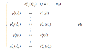
The described procedure deals with such intuitive notions as “frequently occurred” and having “small complexity” sub-formula. In the following algorithms it is supposed that “frequently occurred” means that a sub-formula appears at least twice and “small complexity” means that the number of a sub-formula literals is less then such a number of at least one of the initial formulas.

3.1          Construction of a Level Description of Classes

An algorithm for construction of a level description of classes is presented in [19], [23]. This algorithm contains two parts: 1) extraction of common up to the names of arguments sub-formula from the class description, 2) forming a level description. Here it is presented with more accuracy.

1) Extraction of common up to the names of arguments subformulas from the class description Let the description of a class be A(x) = A₁(x₁) ∨ ··· ∨ A_K(x_K), where A₁(x₁),…, A_K(x_K) are elementary conjunctions of literals.

• For every i and j (i < j) check whether A_i(x_i) ⇒_P ∃x_j, A_j(x_j).

Using the notion of partial sequence we can obtain a maximal common up to the names of arguments sub-formula Q¹_i,j(z¹_i,j) of two elementary conjunctions A_i(x_i) and A_j(x_j) and unifiers λ_Q1i,j,_Ai and λ_Q1i,j,_Aj . Let s_i be the lists of indices of Q^l_si (^zl_si ).

• For l = 1,…, L − 1 do.
• For every s_i and s_j (s_i , s_j) do.

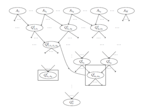
Figure 1: Scheme of common up to the names of arguments sub-formulas extraction.

• In the similar way find a maximal common up to the names

of arguments sub-formula Qls+i,1sj (zls+i,1sj ) of the formulas Qlsi (zlsi ) and Q^l_sj (^zl_sj ) and unifiers ^λ_Qls+i_,1sj ,_Qlsi and ^λ_Qls+i_,1sj ,_Qlsj .

• If a formula Q^l_s⁺_i,¹_sj (^zl_s⁺_i,¹_sj ) is isomorphic to some previously obtained Q^l_s⁰(z^l_s⁰) for some s and l⁰ ≤ l+1 then it is deleted from the set of the (l + 1)th level formulas and we wright down unifiers ^λ_Qls⁰_,Qlsi and λQls0,Qlsj .

Note that the length of Q^l_s⁺_i,¹_sj (^zl_s⁺_i,¹_sj ) decreases with increasing l. That is why the process would stop.

A scheme of the extraction is presented in Figure 1. In order not to overload the scheme, the arguments of the formulas are not written on it and instead of Q^l_si (z^l_si ) it is written Q^l_si  In this scheme it is supposed that highlighted together with its connections formula Q^l_s3,s4 is isomorphic to some previously obtained formula, for example, to Q²_1,i1_,i1_,i2 and that’s why it is deleted from the set of the lth level formulas and all its connections are rewrited to Q21,i1,i1,i2.

A formula Q^l_s⁰_1,s2 that does not have a common sub-formula with any other formulas, is highlighted on it.

2) Forming a level description.

Further, we assume that Q⁰_i (z⁰_i ) is A_i(x_k,i).

• Every formula of the type Q^l_s(z^l_s) which has no sub-formula of the type Q^l_s⁺_,s¹_j (z^l_s⁺_,s¹_j ) for any s_j is declared as P_i¹ (y¹_i ) (i = 1,…,n₁).^[4]

A new 1st level predicate defined as p¹_i (y¹_i ) ⇔ P¹_i (y¹_i ) is introduced and p¹_i (y¹_i ) is substituted (using the correspondent unifies) instead of P¹_i (y¹_i ) into all formulas of the type Q^l_s(z^l_s) (l ≥ 0) such that there is an oriented path from Q^l_s(z^l_s) to P¹_i (y¹_i ).

• For l = 1,…, L − 1 do.

For every i = 1,…,n_l if P^l_i(y^l_i) is a maximal common up to the names of arguments sub-formula of formulas Q^l0 (zl0 ) and Ql0 (zl0 ) then these formulas are declared as P^l_i00⁺¹(y^l_i00⁺¹) and P^l_i00⁺₊¹₁(y^l_i00⁺₊¹₁) (i⁰⁰ = 1,…,n_l+1 − 1).

New (l + 1)th level predicates p^l_i00⁺¹(y^l_i00⁺¹) and p^l_i00⁺₊¹₁(y^l_i00⁺¹) defined as pli00+1(yli00+1) ⇔ Pli00+1(yli00+1) and pli00++11(yli00++11) ⇔ Pli00++11(yil00++11) are introduced and every of them is substituted (using the correspondent

unifies) instead of P^l_i00⁺¹(0 y^l_i00⁺¹) and P_i^l00⁺₊¹₁(y^l_i00⁺₊¹₁), respectively, into all formulas of the type Q^l_s such that there is an oriented path from Q^l_s to at least one of them.

If P^l_i(^yl_i) corresponds to the cell marked as Q²_1,i1_,i1_,i2 in Figure 1 then p^l_i00⁺¹(y^l_i00⁺¹) is substituted instead of P_i^l00⁺¹(y^l_i00⁺¹) into the formulas corresponding the cells marked as Q¹_1,i1, A₁ and A_i1. The literal p^l_i00⁺₊¹₁(y^l_i00⁺₊¹₁) is substituted instead of P^l_i00⁺₊¹₁(^yl_i00⁺₊¹₁) into the formulas corresponding the cells marked as Q¹_i1_,i2, A_i1 and A_i2.

The words “using the correspondent unifies” may be explained in such a way. If P^l_i(^yl_i) corresponds to the cell marked as Q²_1,i1_,i1_,i2 in Figure 1 then p^l_i00⁺¹(y^l_i00⁺¹) is substituted instead of P_i^l00⁺¹(y^l_i00⁺¹) into the formulas corresponding the cells marked as Q¹_1,i1, A₁ and A_i1.

The literal p^l_i00⁺₊¹₁(y^l_i00⁺₊¹₁) is substituted instead of P_i^l00⁺₊¹₁(^yl_i00⁺₊¹₁) into the formulas corresponding the cells marked as Q¹_i1_,i2, A_i1 and A_i2

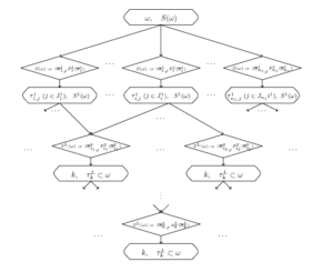
Figure 2: Scheme of level recognition.

It may be easily proved that the problem of level description construction is NP-hard. In particular, the problem of checking if there exists a level description is NP-complete and the upper bounds of number of steps for traditional algorithms exponentially depends on parameters of A₁(x₁),…, A_K(x_K). At the same time such a description must be constructed only once and then may be used as many times as you like.

3.2        The Use of Level Description of a Class

Checking for what k the sequence S(ω) ⇒ ∃x_k,A_k(x_k) is valid and if “yes” then finding for what value of x_k it is valid with the use of level description of a class, may be done according to the following algorithm.

• For i = 1,…,n₁ check S(ω) ⇒ ∃y¹_{i ,}P¹_i (y¹_i ) and find all lists of values τ¹_i,j for the variables y¹_i such that S(ω) ⇒ P_i¹ (τ¹_i,j).^[5]

Let τ¹_i,j be a notation for the list τ¹_i,j. All atomic formulas of the form p¹_i (τ¹_i,j) with τ¹_i,j a notation for the list τ¹_i,j are added to S(ω) to obtain S¹(ω) – a 1st level description of ω.

• For l = 1,…, L − 1 do.
• For i = 1,…,n_l check S ^l ) and find all lists of values τ^l_i,j for the variables y^l_i such that S ^l(ω) ⇒ P^l_i(τ^l_i,j).
• All atomic formulas of the form p^l_i(τ^l_i,j) with τ^l_i,j a notation for the list τ^l_i,j are added to S ^l(ω) to obtain S¹⁺¹(ω) – a lth level description of ω.
• – For k = 1,…, K check S ^L(ω) ⇒ ∃y_k^L_,A_k^L(y_k^L) and find all lists of values ^τ_k^L_,j for the variables y_k^L such that S ^L(ω) ⇒ A_k^L(^τ_k^L_,j).

The object ω satisfies such formulas A_k(x_k) for which the corresponding sequence S ^L(ω) ⇒ ∃y_k^L_,A_k^L(y_k^L) is valid.

The scheme of level recognition is presented in Figure 2.

It is proved in [8] that for a two-level description (L = 1) the number of steps with the use of 2-level description decreases. For an exhaustive algorithm the number of steps decreases from O(t^mk ) to O(n₁ · t^r + t^δ1_k⁺ⁿ¹), where r is a maximal number of arguments in the 1st level predicates, n₁ is the number of such predicates, δ¹_k is the number of initial variables which are presented in A_k(x_k) and are absent in A¹_k(x¹_k). Both parameters r and δ¹_k + n₁ are less than m_k.

Number of steps for an algorithm based on the derivation in predicate calculus decreases from O(s_k^ak ) to O(s^1a1k + ^Pn_j=¹₁ s^ρ1j ), where a_k and a¹_k are maximal numbers of literals in A_k(x_k) and A¹_k(x¹_k), respectively, s and s¹ are the numbers of literals in S(ω) and S¹(ω), respectively, ρ¹_j is the numbers of literals in P¹_i (y¹_i ). Both parameters a¹_k and ρ¹_j are less than a_k.

So, the recognition of an object with the use of a level description requires less time than that with the use of initial description.

4. Logic-Predicate Network

The inputs of a traditional neuron network are binary or many-valued characteristics of an object. The neuron network configuration is fixed that does not correspond to biological networks.

Below a logic-predicate network is described. Such a network inputs are atomic formulas setting properties of the elements composing an investigated object and relations between them [17], [19]. Further it will be shown that its configuration may be changed during its retraining.

A level description of a class of objects permits quickly enough to recognize an object which description is isomorphic to the description of an element of a training set.

A logic-predicate network consists of two blocks: a training block and a recognition block. Training block forms a level description of a class of objects according to a training set (or some formalized description of the class). Its content is presented in Figure 1.

Recognition block implements the algorithm of the use of level description of a class. It must be marked that the level description may be represented as an oriented graph presented in Figure 2.

Scheme of logic-predicate network is presented in Figure 3. Here inputs and outputs are situated in ovals and checking the conditions are situated in rhombus.

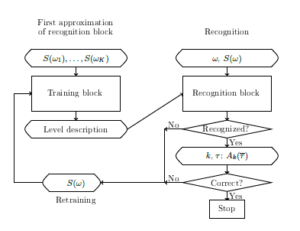
Figure 3: Scheme of logic-predicate network.

Let a training set of objects ω¹,…,ω^K be given. An initial variant of the class description may be formed by replacement of every constant ω^k_j in S(ω^k) by a variable x^k_j (k = 1,…, K, j = 1,…,t^k) and substitution of the sign & between the atomic formulas. Construct a level description for these goal formulas. The first approximation to the recognition block is formed.

If after the recognition block run an object is not recognized or has wrong classification, then it is possible to retrain the network. The description of the “wrong” object must be added to the input set of the training block. The training block extracts common up to the names sub-formulas of this description and previously received formulas forming a new recognition block. Some sub-formulas, the number of layers and the number of formulas in every layer may be changed in the level description. Then the recognition block is reconstructed.

5. Example of Logic-Predicate Network Construction, its Running and Retraining

Let a set of contour images of “boxes” be to recognize. Every image may be described in the terms of two predicates V and L defined as it is presented in Figure 4.

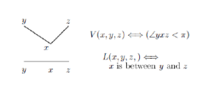
Figure 4: Initial predicates.

A training set {ω₁,ω₂,ω₃} of such images is presented in Figure

5. Here ω₁ = {a₁,…,a₁₀}, ω₂ = {b₁,…,b₈}, ω₃ = {c₁,…,c₁₀}.

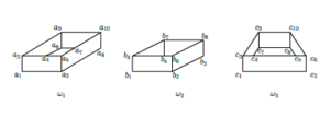
Figure 5: Training set.

In order not to overload the text, we write down only the formula A₂(y₁,…,y₈), which is obtained from the description S(ω₂) by replacing the names b_i with the variables y_i and placing the sign & between the literals.

A₂(y₁,y₂,y₃,y₄,y₅,y₆,y₇,y₈) =

V(y₁,y₄,y₂) & V(y₂,y₁,y₆) & V(y₂,y₁,y₃) & V(y₂,y₆,y₃) & V(y₃,y₂,y₈) & V(y₄,y₇,y₆) & V(y₄,y₇,y₅) & V(y₄,y₇,y₁) & V(y₄,y₅,y₁) & V(y₄,y₆,y₁) & V(y₅,y₄,y₇) & V(y₅,y₄,y₆) &

V(y₅,y₇,y₆) & L(y₅,y₄,y₆) & V(y₆,y₄,y₈) & V(y₆,y₅,y₈) &

V(y₆,y₈,y₂) & V(y₆,y₂,y₅) & V(y₆,y₂,y₄) & V(y₇,y₄,y₅) &

V(y₇,y₅,y₈) & V(y₇,y₄,y₈) & V(y₈,y₃,y₆) & V(y₈,y₆,y₇) & V(y₈,y₃,y₇)

Further, for clarity, we will write down not formulas, but drawings.

5.1        Training Block Run: Extraction of Sub-Formulas

For constructing a level description, find pairwise maximal common up to the names of arguments sub-formulas Q¹_i (y¹_i ) of formulas A₁(x), A₂(y), A₃(z) and their unifiers. See Figure 6.

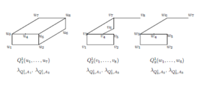
Figure 6: First extraction of pairwise maximal common up to the names of arguments sub-formulas.

Here the following unifier are formed.

Let u¹ = (u₁,…,u₈), v¹ = (v₁,…,v₈), w¹ = (w₁,…,w₇). λ_Q11,_A1 = (u₁ → x₁,u₂ → x₂,u₃ → x₃,u₄ → x₄,u₅ → x₅,u₆ →

x8,u7 → x9,u8 → x10) = (u1 → x11), λ_Q11,_A2 = (u₁ → y₁,u₂ → y₂,u₃ → y₄,u₄ → y₅,u₅ → y₆,u₆ →

y₃,u₇ → y₇,u₈ → y₈) = (u¹ → y¹₁), λ_Q12,_A1 = (v₁ → x₁,v₂ → x₂,v₃ → x₃,v₄ → x₄,v₅ → x₅,v₆ →

x6,v7 → x9,v8 → x10) = (v1 → x21), λ_Q12,_A3 = (v₁ → z₁,v₂ → z₂,v₃ → z₃,v₄ → z₄,v₅ → z₆,v₆ →

z7,v7 → z9,v8 → z10) = (v1 → z11),

λ_Q31,_A2 = (w₁ → y₁,w₂ → y₂,w₃ → y₄,w₄ → y₅,w₅ → y₆,w₆ → y₇,w₇ → y₈) = (w¹ → y¹₂), λ_Q31,_A3 = (w₁ → z₁,w₂ → z₂,w₃ → z₃,w₄ → z₄,w₅ → z6,w6 → z9,w7 → z10) = (w1 → z12).

Pairwise extractions of maximal common up to the names of arguments sub-formulas of Q¹₁(u₁,…,u₈), Q¹₂(v₁,…,v₈) and Q¹₃(w₁,…,w₆) give only just obtained formula Q¹₃(w₁,…,w₆). That’s why we have a situation presented in Figure 7.

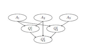
Figure 7: Connections between the extracted formulas.

5.2        Training Block Run: Forming a Level Description

The formula Q¹₃(w₁,…,w₇) has no common sub-formulas with the other ones. Therefore, it is the 1st level predicate P¹₁(w₁,…,w₇) of the network. A new 1st level predicate p¹₁(w¹) defining as p¹₁(w¹) ⇔ P¹₁(w₁,…,w₇) is introduced. Remind that w¹ is a new 1st level variable for the string of initial variables (w₁,w₂,w₃,w₄,w₅,w₆,w₇).

Formula P¹₁(w₁,…,w₇) (which corresponds to Q¹₃(w₁,…,w₇)) is on the end of edges from A₂(y₁,…,y₈), Q¹₁(u₁,…,u₈) and Q¹₂(v₁,…,v₈) in Figure 7. The unifier of P¹₁(w₁,…,w₇) with A₂(y₁,…,y₈) coincides with λ_Q13,_A2 obtained above.

The unifiers of P¹₁(w₁,…,w₇) with Q¹₁(u₁,…,u₈) and Q¹₂(v₁,…,v₈) are the following.

λ_P11,_Q11 = (w¹ → u²), where u² = (u₁,u₂,u₃,u₄,u₅,u₇,u₈). λ_P11,_Q12 = (w¹ → v²), where v² = (v₁,v₂,v₃,v₄,v₅,v₇,v₈).

The formulas Q¹₁(u₁,…,u₈) and Q¹₂(v₁,…,v₈) with the substitutions of p¹₁(u¹) and p¹₁(v¹), respectively, instead of sub-formulas isomorphic to P¹₁(w₁,…,w₇) will form the 2nd level of the network and are denoted by P²₁(u₁,…,u₈;u¹) and P²₂(v₁,…,v₈;v¹).

It must be marked that if we know the value of the 1st level variable u¹ then we know the values of (u₁,u₂,u₃,u₄,u₅,u₇,u₈). That’s why the essential variables of P²₁(u₁,…,u₈;u¹) are (u₆;u¹). Similarly the essential variables of P²₂(v₁,…,v₈;v¹) are (v₆;v¹).

New 2nd level predicates p²₁(u²) and p²₂(v²) defining as p²₁(u²) ⇔ P²₁(u₁,…,u₈;u¹) and p²₂(v²) ⇔ P²₂(v₁,…,v₈;v¹) are introduced.

Taking into account only essential variables and earlier received unifiers we have the last layer formulas.

A²₁,₁(x₇; x¹, x₁²), where x¹ = (x₁, x₂, x₃, x₄, x₅, x₈, x₉, x₁₀), x₁² = (x₆; x¹).

A²₁,₂(x₇; x¹, x₂²), where x¹ = (x₁, x₂, x₃, x₄, x₅, x₈, x₉, x₁₀), x₂² = (x₆; x¹).

A²₂,₁(;y¹,y²₁), where

y¹ = (y₁,y₂,y₄,y₅,y₆,y₇,y₈), y²₁ = (y₃,y₈;y¹).

A²₂,₂(y₃y₇;y¹), where y¹ = (y₁,y₂,y₄,y₅,y₆,y₇,y₈).

A²₃(z₅,z₈;z¹,z²), where z¹ = (z₁,z₂,z₃,z₄,z₆,z₉,z₁₀), z² = (z₄,z₇;z¹).

The contents of the last layer cells are the following:

5.3        Recognition Block Run

The recognition block is formed according to the level description constructed in the previous subsection. The scheme of recognition block is presented in Figure 8. In this scheme only names of a checking formula and results of checking are written down.

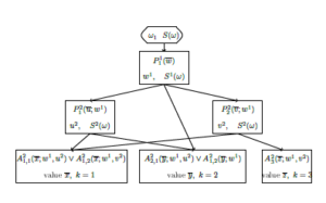
Figure 8: Predicate network.

It is obvious that if an input object ω is isomorphic to one from the training set, then it will be recognized. It means that the number k and such a permutation ω of ω that S(ω) ⇒ A_k(ω) will be found.

Let a control object with the description not isomorphic to anyone from the training set is to be recognized. Such a control object {d₁,…,d₈} is presented in Figure 9.

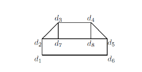
Figure 9: Control object.

Checking S ) in the first layer (see Figure 8) gives us w = (d₁,d₆,d₂,d₇,d₅,d₃,d₄). A new 1st level variable w¹ takes this list of constants as a value. Add new atomic formula to S(ω) and obtain S .

Neither P ) or P ) are a consequence of S¹(ω) be-cause, in fact, 7 variables in u and v are changed by constants from w1.

This control object is not recognized.

5.4          Retraining the Network

Let’s retrain the network with the object presented in Figure 9.

Replace every constant d_i (i = 1,…,8) in its description by a variable x_i and substitute the sign & between the atomic formulas. The formula A₄(x) is obtained.

Pairwise checking of partial sequence between A₄(x) and A_j(x_j) (j = 1,2,3) permits to obtain maximal common up to the names of arguments formulas Q¹₄, Q¹₅ and Q¹₆. The images of thees fragments are shown in Figure 10.

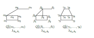
Figure 10: Pairwise extraction of maximal common up to the names of arguments sub-formulas between A₄(x₄) and A_j(x_j) (j = 1,2,3).

One of the obtained formulas (formula Q¹₄(α₁,…,α₇)) is isomorphic to the earlier obtained formula Q¹₃(w₁,…,w₇). That’s why it would not be added to the 2nd layer of the retrained network. But all its connections with the cells of another layers would be saved.

Pairwise checking of partial sequence between Q¹₅, Q¹₆ and Q¹_j(x¹_j) (j = 1,2,3) does not give any new formulas.

So, the 1st layer would have only the formula Q¹₃(w₁,…,w₇) renamed as P¹₁(w₁,…,w₇).

On the 2nd layer the cell with formula P²₄(β;w¹) and output t² and the cell with formula P²₅(γ;w¹) and output r² would be added on the end of the edge from the cell with P¹₁(w). Edges from these cells to the cells with A²_j(x_j; x¹_j, x²_j) (j = 1,2,3) would be added as it is shown in Figure 11.

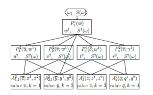
Figure 11: Pairwise extraction of maximal common up to the names of arguments sub-formulas between A₄(x₄) and A_j(x_j) (j = 1,2,3).

The network is retrained.

It should be noted that the examples of images discussed in the article are taken from [3]. The original predicates W, Y and T in that book for describing the images differ from the predicates V and L used here. This is due to the fact that W, Y and T are expressed in terms of the predicates V and L and do not significantly reduce the computational complexity of recognition when constructing a level description.

Both {W, Y, T} and {V, L} are not enough to describe real images of “boxes”. So, for example, the description of the image in Figure 12 is isomorphic to the description of A₂(y₁,…,y₈), but you need to have a rich imagination to guess the box in it. The choice of initial predicates in each specific problem should be chosen very carefully.

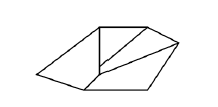
Figure 12: Is it a box?

Here we do not consider an example when, while retraining the network, not only additional cells in a layer appear, but the number of layers also changes. This could be done by retraining the network using the example of a mirror (relative to the vertical axis) image of an object from the training set. In this case, rectangle recognition will appear in the 1st layer. The contents of the remaining cells will also be changed.

6. Fuzzy Recognition by a Logic-Predicate Network

The disadvantage is that the proposed logic-predicate network does not recognize objects with descriptions that are not isomorphic to the descriptions that participate in its formation. This can be eliminated by slight modifications of the network.

Further the ith cell of the lth level will be denoted as cell_i^l.

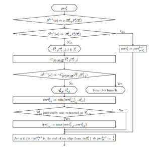
Figure 13: The fuzzy network ith cell of the lth level contents.

Let’s change the contents of the network cells presented in Figure 2 by replacing the checking of S ^l−1(ω) ⇒ ∃x^l_i,P^l_i(x^l_i) in the cell_i^l with the partial sequence checking S ^l−1(ω) ⇒_P ∃x^l_i,P^l_i(x^l_i). The degree of coincidence of a recognized object with the description of a class and the degree of recognition correctness certainty is calculated during partial sequence checking.

For a fully identified object, both of these degrees equal to 1. For an object from a given class for which these degrees are essentially small (this is determined by an expert), you can still retrain the network.

A fuzzy network has two additional parameters:

cert_i^l (l = 0,…, L, i = 1,…,n_l) – a degree of certainty in the correctness of recognition by the cell_i^l;

pre^l_i ( l = 1,…, L, i = 1,…,n_l) – the cell number of a cell preceding the cell_i^l in the current traversal of a network. The cell0 number has the form ^l_j , where l⁰ is the number of a layer and j is the number of a cell in this layer Initially, cert₁⁰ := 1, pre¹_i := ⁰₁ (i = 1,…,n₁).

The scheme of cell_i^l contents of a fuzzy network is presented in Figure 13.

First of all, a partial sequence S ^l−1(ω) ⇒_P ∃x^l_i,P^l_i(x^l_i) is checked in this cell. If this sequence is not partial but total, then the parameter cert_i^l is not changed and the calculation goes to the end of the cell.

Otherwise, all lists of constants τ^l_{i j} and maximal not contradictory on τ^l_{i j} with S ^l−1(ω) sub-formulas P_e^l_{i j}(x^l_{i j}) of the formula P^l_i(x^l_i) are found while partial sequence checking.

If the sub-formulas P_e^l_{i j}(x^l_{i j}) is contradictory to the description S(ω) on the list of the found constants, then this recognition branch stops.

Remind that S(ω) and C_[Pli(_xli)]τx⁰ P_e^l_{i j}(τ^l_{i j}) are in the contradiction means that S(ω) ⇒ ¬C[Pli(xli)]τx0 Peli j(τli j), where C[Pli(xli)]τx0 Pei jl (τi jl ) is a complement (conjunction of literals from P^l_i(x^l_i) which are not in Peli j(xli j)) of Peli j(xli j) up to Pli(xli).^[6]

Parameters q^l_{i j} and r_{i j}^{l [7]} are calculated with the use of the full form of formulas P^l_i(x^l_i) and P_e^l_i(y^l_i), i.e., with the replacement in them of each atomic formula of the levels l⁰ (l⁰ < l) by the defining elementary conjunction.

Except this, a degree of certainty cert_i^l that the recognition would be valid is calculated in every cell. While first visit to the cell_i^l the value of cert_i^l will be cert_i^l := min{cert¹_pre⁻¹_li ,q^l_i}. This corresponds to conjunction of degrees of certainty while successive passage along one branch of network traversal.

While next visit of the cell_i^l the value of cert_i^l will be cert_i^l := max{cert_i^l,min{cert¹_pre⁻¹_li ,q^l_i}}. This corresponds to disjunction of degrees of certainty while parallel passage along different branches of network traversal.

Why can we visit a cell not only once? For example, in Figure 11 the 3rd layer cell with A²₁ may be visited by a path including the cells with P¹₁, P²₁ and A²₁ and by a path including the cells with P¹₁, P22 and A21.

In the last layer of the network, objects ^τ_k^L would be received and for each object the degree of certainty q_k^L, that it is the r_k^Lth part of an object satisfying the description A_k(x_k), would be calculated.

A flowchart of fuzzy recognition network can not be presented in the paper because it is very large. It consists of the “Scheme of logic-predicate network” shown in Figure 3, in which instead of the “Training block” the “Scheme of common up to the names of

arguments sub-formulas extraction” (Figure 1) is inserted, and the “Scheme of level recognition” (Figure 2) is inserted instead of the “Recognition block”. At the same time, in Figure 2, each element enclosed in a rhombus is replaced by “The fuzzy network ith cell of the lth level contents” (Figure 13).

7. Model Example of Fuzzy Recognition

Let’s look how a fuzzy network (corresponding to that constructed in the section 6 and presented in Figure 8) recognizes the control object presented in Figure 9.

To recognize it, a partial sequence S(d₁,d₂,…,d₈)               ⇒_P ,…,w₆) is checked in the 1st layer. There is a total sequence and the 1st level variable w¹ = (w₁,w₂,w₃,w₄,w₅,w₆,w₇) takes the value (d₁,d₆,d₂,d₇,d₅,d₃,d₄). cert11 := 1, pre21 := 11, pre22 := 11, pre32 := 11.

The result of the 1st layer fuzzy cell run is presented in Figure 14.^[8]

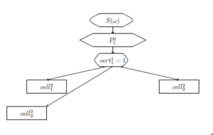
Figure 14: The result of the 1st layer fuzzy cell run.

In the 2nd layer, partial sequence S¹(d₁,d₂,…,d₈,w¹) ⇒_P ) is checked. It must be noted that in fact S¹(d₁,d₂,…,d₈,w¹) ⇒_P ∃u ) is checked. That is, there is only one variable at the right-hand side of the formula.

Since we need to check formulas for consistency, we note that V(x,y,z) ⇒ ¬V(x,z,y).

There is only a partial sequence. A formula P˜²₁(d₁,d₆,d₂,d₇,d₅,d₃,d₄;w¹) is the maximal sub-formula such that S¹(d₁,d₂,…,d₈,w¹) ⇒ P˜²₁(d₁,d₆,d₂,d₇,d₅,d₃,d₄;w¹). Its complement up to P²₁(d₁,d₆,d₂,d₇,d₅,d₃,d₄,u₆;w¹) contains three literals with predicate V, one of them is V(u₆,d₄,d₆). This contradicts S¹(d₁,d₂,…,d₈,w¹) containing V(u₆,d₆,d₄). This branch of the network stops.

There is another cell in the 2nd layer on the end of an edge from cell₁¹. This is cell₂². Check      partial     sequence         S¹(d₁,d₂,…,d₈,w¹)                 ⇒_P ).   In fact, S¹(d₁,d₂,…,d₈,w¹)     ⇒_P ) is checked.

There is only partial sequence. A formula P˜²₂(d₁,d₆,d₂,d₇,d₅, v₆,d₃,d₄;w¹) is the maximal sub-formula such that S¹(d₁,d₂,…,d₈,w¹) ⇒ P˜ ). Its complement up to P ) contains 5 literals with predicate V V(v₆,d₇,d₃), V(d₃,v₆,d₂), V(d₇,v₆,d₂), V(d₇,d₈,v₆), V(d₇,d₅, v₆) and 3 literals with predicate L

L(d₇,d₂,d₈), L(d₈,d₂,d₅), L(d₈,d₇,d₅), but no one of them is in contradiction with S¹(d₁,d₂,…,d₈,w¹). The value of v² is (v₆;w¹).

It means that one 1st level variable v₆ does not take value.

The number of literals in P²₂(v₁ …v₈;w¹) (taking into account its full form in which the 1st level predicate is changed by the defining formula only with initial variables) is a²₂ = 16. The number of literals in P˜²₂(d₁,d₆,d₂,d₇,d₅,v₆,d₃,d₄;w¹) is ˜a²₂ = 8.

That’s why q²₂ = = and cert₂² := min{1, } = .

There are two edges from the cell with P²₂ to the 3rd layer cells with A²₁,₂ and with A²₃. That’s why pre³₁ := ²₂, pre³₃ := ₂².

The result of the 2nd layer fuzzy cells run is presented in Figure 15.

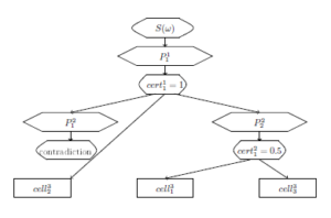
Figure 15: The result of the 2nd layer fuzzy cell run.

In the 3rd layer while going from the cell with P¹₁ to the cell₂³ with A²_2,1 partial sequence S¹(d₁,…,d₈;w¹) ⇒_P ) is checked. In fact, a partial sequence S¹(d₁,…,d₈;w¹) ⇒_P ) with the only one initial variable y₃ is checked.

There is only a partial sequence. The same string of values for variables in v², as it was in the second layer, partially satisfies A ). But the description of this fragment has two additional literals V(d₇,d₂,d₃) and V(d₇,d₃,d₅).

The number of literals in A₂(y₁ …y₈; v¹) is a₂ = 22. The number of literals in A˜²_1,2(y₁ …y₈;v¹,v²) is a˜²_1,2 = 10. That’s why q 455 and cert

While going from the cell with P²₂ to the cell₁³ with A²_1,2 partial sequence S²(d₁,d₂,…,d₈;v¹,v²) ⇒_P )        is             checked.                In             fact S²(d₁,d₂,…,d₈;v¹,v²)      ⇒_P                       , v₇,v₈,d₃,d₄;v¹,v²) with 3 initial variables v₆, v₇, v₈ is checked.

There is only a partial sequence. The same string of values for variables in v², as it was in the second layer, partially satisfies A21,2(v1 …v10;v1,v2).

The number of literals in A₁(x₁,…, x₁₀) is a₁ = 34. The number of literals in A˜ ) is a˜   8.       That’s why235 and cert While going from the cell with P cell₂³ with A²₃ partial sequence S²(d₁,d₂,…,d₈;v¹,v²) ⇒_P is checked. In fact S²(d₁,d₂,…,d₈;v¹,v²) ⇒_P ) with 2 initial variables z₇, z₈ is checked.

There is only a partial sequence. The variables z₇, z₈ have not taken values. All literals with these variables are absent in A˜²₃(d₁,d₆,d₂,d₇,d₈,d₅,z₇,z₈,d₃,d₄;v¹,v²). The number of such literals is 14.

The number of literals in A is a₃ = 32. The number of literals in A˜ ) is a˜          18. That’s why q     563 and cer The full degree of certainty that it is a representative of the class of “boxes” that is given as a control image is cert =

Moreover, elements of this image coincide with elements of the image ω₃ from the training set.

The result of the fuzzy network run is presented in Figure 16.

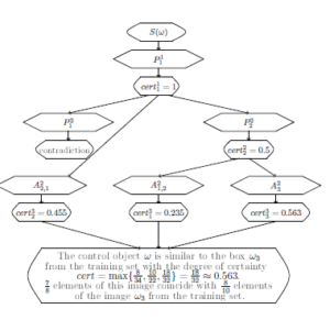
Figure 16: The result of the fuzzy network run.

8. Results and Discussion

The main result of this article is the proposal of fuzzy recognition of complex structured objects by logic-predicate network. For a detailed presentation of this result, it was necessary to describe in detail a logic-predicate approach to the recognition of complex structured objects.

A significant disadvantage of this approach is that the problems arising are NP-hard, which to a large extent “scares off” some researchers. On the other hand, the use of predicate logic does not always seem legitimate, since the propositional logic is much simpler for understanding by non-mathematicians.

The use of level descriptions is not something essentially original to decrease the computational complexity of the main problem. It is a well-known technique in which sufficiently complex problems are divided into a sequence of problems of the same type of lower dimension. The main problem was HOW to build such a description. To this end, the mathematical apparatus for extracting the general sub-formulas of two elementary conjunctions of predicate formulas was developed and briefly presented in this paper.

Based on the level description of classes, it was possible to formulate the concept of a logic-predicate network. Unlike existing networks, for example, neural or Bayesian, when retraining such a network, a logic-predicate network can (and, as a rule, this happens) change its configuration. This corresponds to the training of a person in whose brain connections between one neural cells break and connections between others arise.

This is one of the essential features of the proposed approach, which distinguishes it from the use of various other networks. Its other essential feature is to calculate the degree of coincidence of the object being recognized with those ones for which the network was trained.

A trained logic-predicate network quickly recognizes objects with descriptions that are isomorphic to the ones on which it was trained. But its training and retraining processes remain to be NPhard. This corresponds to the process of teaching a person. But in some cases, it is not necessary to accurately recognize an object or process, but to find out what it looks like and to what extent.

To answer such a question, the concept of a fuzzy logic-predicate network was proposed. The structure of its cell, shown in Figure 13, is quite complex and contains a partial sequence check. Such verification is NP-hard, but after repeated retraining of the network, the formulas P^l_i(x^l_i), setting intermediate goal formulas, are quite short and have a small number of essential arguments, as it was shown by the example in section 7. This means that an exponent of the computational complexity of the partial sequence check is a fairly small value.

Special importance has the choice of “good” initial features. As already mentioned in Subsection 5.4, the predicates W, Y and T, which were used to describe contour images in [3], do not give a good decreasing of computational complexity for the logic-predicate network, constructed from them. Apparently, this is due to the fact that they reflect the perception of a person and are essentially composite.

9. Conclusion

In development of the proposed approach, many-valued predicates may be considered. Especially this relates to the properties of an object elements. Such multi-valued predicates p(x) = a with a ∈ D can be interpreted as binary ones with a numerical argument: q(x;a) ⇔ p(x) = a. The inclusion of such predicates in the formulation of the problem may serve as the subject of further research.

It is also planned to consider the possibility of introducing cell weights in a logic-predicate network. Such weights can be determined depending on the frequency with which parts of an object description satisfy the formula checked in the corresponding cell. Other weighting strategies are possible, similar to strategies for determining the cell weights of a classical artificial neural network.

In addition, if in the problem setting global features of the object that characterize the entire object are considered, then such an object is usually described by a binary or multi-valued string. Class descriptions can be presented as a propositional formula in disjunctive normal form. Extraction the “frequently encountered” sub-formulas of such propositional formulas [24] allows to form a level description of classes. Using this description in a manner similar to that described in this article, it is possible to build a logicalgebraic network, which changes its configuration in the process of learning. This corresponds to a change of connections in biological neural networks.

Acknowledgments

The    author    is     grateful    to      Vakhtang Kvaratskhelia from Muskhelishvili Institute of Computational Mathematics of the Georgian Technical University, whose question at the conference in 2017 allowed this paper to be born. The author thanks the anonymous referees for their useful suggestions.

1. T. Kosovskaya . “Implementation of Formula Partial Sequence for Rough Solution of AI Problems in the Framework of the Logic-Predicate Approach” in 2019 Computer Science and Information Technologies (CSIT),Yerevan,
   Armenia, 2019. https://doi.org/10.1109/CSITechnol.2019.8895153
2. N. J. Nilson, Problem-solving methods in Artificial Intelligence, McGraw-Hill Book Company, 1971.
3. R. Duda, P. Hart, Pattern Classification and Scene Analysis, John Wiley & Sons, 1973.
4. E.B. Hunt, Artificial Intelligence, Academic Press, 1975.
5. M.R. Garey, D.S Jonson, Computers and Intractability: A Gide to the Theory of NP-Completeness, W.H. Freeman and Company, 1979.
6. S. Russell, P. Norvig, Artificial Intelligence: A Modern Approach, Third edition, Prentice Hall Press Upper Saddle River, 2009.
7. T.M. Kosovskaya. ”Estimating the number of steps that it takes to solve some problems of pattern recognition which admit logical description” in VESTNIK ST PETERSBURG UNIVERSITY-MATHEMATICS, 40(4), 82–90, 2007. (In Russian) https://doi.org/10.3103/S1063454107040061
8. T.M. Kosovskaya, ”Multilevel descriptions of classes for decreasing of step number of solving of a pattern recognition problem described by predicate cal- culus formulas” VESTNIK SANKT-PETERBURGSKOGO UNIVERSITETA SERIYA 10 PRIKLADNAYA MATEMATIKA INFORMATIKA PROTSESSY, 1, 64–72 (2008). (In Russian)
9. T.M. Kosovskaya, ”Partial deduction of predicate formula as an instru- ment for recognition of an object with incomplete description” VESTNIK SANKT-PETERBURGSKOGO UNIVERSITETA SERIYA 10 PRIKLAD- NAYA MATEMATIKA INFORMATIKA PROTSESSY, 1, 74–84, 2009. (In Russian) https://doi.org/10.24412/FgeTsEutG6w
10. T.M. Kosovskaya, “Partial Deduction in Predicate Calculus as a Tool for Artificial Intelligence Problem Complexity Decreasing” in 2015 IEEE 7th International Conference on Intelligent Computing and Information Systems,
    ICICIS 2015, 73–76, 2016. https://doi.org/10.1109/IntelCIS.2015.7397199
11. J. Schmidhuber, “Deep learning in neural networks: An overview” Neural Networks, 61, 85–117, 2015. https://doi.org/10.1016/j.neunet.2014.09.003
12. T. Chunwei, X. Yong, Z. Wangmeng, “Image denoising using deep CNN with batch renormalization” Neural Networks, 121, 461–473, 2020. https://doi.org/10.1016/j.neunet.2019.08.022
13. E.H. Dawn, C. J. Lakhmi (Eds), Innovations in Bayesian Networks. Theory and Applications, Springer-Verlag, 2008. https://doi.org/10.1007/978-3-540-85066-3
14. R. Agrahari, A. Foroushani, T.R. Docking et al. “Applications of Bayesian network models in predicting types of hematological malignancies”, Sci Rep 8, 6951 (2018). https://doi.org/10.1038/s41598-018-24758-5
15. A. Tulupiev, C. Nikolenko, A. Sirotkin, Bayesian Networks: logic-probabilistic approach, Nauka, 2006. (in Russian)
16. A. Shahzad, R. Asif, A. Zeeshan, N. Hamad, A. Tauqeer, “Underwater Resur- rection Routing Synergy using Astucious Energy Pods” Journal of Robotics and Control (JRC), 1(5), 173–184, 2020. https://doi.org/10.18196/jrc.1535
17. T. Kosovskaya, “Self-modificated predicate networks” International Journal on Information Theory and Applications, 22(3), 245–257, 2015.
18. T. Kosovskaya, “Fuzzy logic-predicate network” in Proceedings of the 11th Conference of the European Society for Fuzzy Logic and Technology (EUSFLAT 2019), Part of series ASUM (Atlantis Studies in Uncertainty Modeling), 1, 9–13, 2019. https://doi.org/10.2991/eusflat-19.2019.2
19. T. Kosovskaya, “Predicate Calculus as a Tool for AI Problems Solution: Algorithms and Their Complexity”, 1–20. 2018. Chapter 3 in “Intelligent System”, open-access peer-reviewed Edited volume. Edited by Chatchawal Wongchoosuk Kasetsart University https://doi.org/10.5772/intechopen.72765
20. T. M. Kosovskaya, N. N. Kosovskii, “Polynomial Equivalence of the Problems Predicate Formulas Isomorphism and Graph Isomorphism” VESTNIKST PETERSBURG UNIVERSITY-MATHEMATICS, 52(3), 286–292, 2019.
    https://doi.org/10.1134/S1063454119030105
21. T.M. Kosovskaya, “Some artificial intelligence problems permitting formalization by means of predicate calculus language and upper bounds of their solution steps” SPIIRAS Proceedings, 14, 58–75, 2010. (In Russian) https://doi.org/10.15622/sp.14.4
22. T. M. Kosovskaya, D. A. Petrov, “Extraction of a maximal common sub-formula of predicate formulas for the solving of some Artifi- cial Intelligence problems” VESTNIK SANKT-PETERBURGSKOGO UNIVERSITETA SERIYA 10 PRIKLADNAYA MATEMATIKA INFORMATIKA PROTSESSY, 3, 250–263, 2017. (In Russian) https://doi.org/10.21638/11701/spbu10.2017.303
23. T. Kosovskaya, “Construction of Class Level Description for Efficient Recognition of a Complex Object” International Journal “Information Content and Processing”, 1(1), 92–99, 2014.
24. D.A. Koba, “Algorithm for constructing a multi-level description in pattern recognition problems and estimating the number of its run steps” in Proceedings of the XVII International School-Seminar “Synthesis and Complexity of Control Systems” named after Acad. O.B. Lupanov (Novosibirsk, October 27 – November 1, 2008), Publishing House of the Institute of Mathematics, Novosibirsk, 55–59, 2008. (In Russian)

(Click Here)

(Click Here)