1. Introduction

The World Health Organization (WHO) in 2013 reported that road traffic accidents that result to loss of lives and damages to properties will continue to become a global challenge due to rapid motorization and insufficient action of national governments [1]. In the Philippines, traffic accidents are mainly due to driver’s error [2] or violation [3] and this prompts government agencies to focus on regulation of driver by means of licensing and provide safer roads by building infrastructures like traffic lights and signs. Another solution includes the development of advanced driver-assistance systems (ADAs) that enhance vehicle systems to aid drivers on the different weather phenomenon and road conditions [4] that degrades their effectivity [5]. This can be solved by employing more complex algorithms but this has an adverse effect to processing speed that is a must for smart vehicle systems. This trade-off between system accuracy and speed is still the biggest challenge in the implementation of ATSDR systems.

This paper “Real-Time Traffic Sign Detection and Recognition System for Assistive Driving” is an extension of work originally presented by the authors in International Symposium on Multimedia and Communication Technology (ISMAC) 2019 entitled “Traffic Sign Detection and Recognition for Assistive Driving” [6]. The goal of this study is to help solve the problem of drivers neglect and lack of road education by implementing an ATSDR system that automatically detects and recognizes road traffic signs then provides information to the driver about the meaning of the signs. This work is the full implementation of a study that the previous work [6] is a part of. The differences between this work and the previous work include (1) gathering and utilization of new traffic road image dataset and road sign image datasets for training and testing the system, (2) evaluation of four pre-processing and detection methods for the detection stage, (3) addition of a Convolutional Neural Network (CNN) deep learning algorithm in the evaluation for the recognition stage aside from the original nine methods, (4) the detection and recognition methods are evaluated not only using the segmentation and classification success rate (accuracy) metric but also processing speed, (5) system-level optimization is done to improve accuracy by fine-tuning sub-processes and a negative class is added to reduce false detection, (6) the models are fully implemented not only in a personal computer but in an embedded system using microcomputer with interface camera, display and speaker, and (7) the system installed in a sedan car is tested in an actual road setup.

Traffic signs defined by the Department of Public Works and Highways to be recognized must be strategically positioned, clear and fully visible [7] and captured in good weather condition during daytime and will be limited only to six regulatory signs corresponding to speed limit, no overtaking and no turning shown in Figure 1. These are generally characterized by their red circular boundaries. The detection and recognition will only be limited to a single traffic sign in a single video frame. The capturing device will be installed to a sedan car with a target maximum speed of at least sixty (60) kilometers per hour. The system will be able to provide voice alert to the driver before the car completely passed by the traffic sign. Implementation of the system will make use of methods from previous studies using Python and open-source libraries.

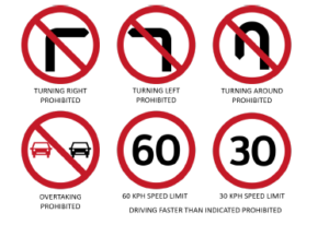
Figure 1: Traffic signs to be recognized

Several implementations of traffic sign detection and recognition systems used different algorithms in pre-processing, detection and recognition phases. Pre-processing stage is necessary to suppress noise and improve image performance [8]. A study [6] showed the detection improvements in traffic sign recognition provided by the use of pre-processing and filtering methods by means of contrast stretching, color normalization and image enhancement before getting the regions of interest. Other techniques are applied depending on the choice of segmentation method in the detection stage which can be color-based, shape-based or combination of both, though color-based is widely implemented in the detection of road signs [9]. Shape based segmentation may have problem when there are similar objects to the traffic signs. It can be quite computationally expensive, and by nature, sensitive to noise. Many shape detectors are slow in computing over large and complex images [10] which will become an issue in a real-time system. The complexity of color based lies in the usage of three intensity values depending on the color space instead of just working in gray level image as in shape based. But still, color segmentation is used more often as color usually provides enough information on the meaning of the traffic sign to be recognized than shape segmentation. Difficulties in color-based detection include lack of standard colors among countries, and various phenomenons and different imaging conditions that cause color variations. In these cases, traffic sign images may appear with varying illumination, blurred, faded, highlighted, noisy, and physically damaged [5] affecting the performance of the color segmentation process. A study [11] solved this problem by instead of working on absolute RGB values, relative RGB values are used for they are almost unchanged with various illumination circumstances. Another study [8] combined four color spaces namely RGB, HSV, YIQ, and XYZ based on histogram to provide more accurate segmentation. Color is segmented using K-means clustering and effective robust kernel based Fuzzy C-means clustering resulting to a more accurate segmentation but has increased computational complexity. In [10], color segmentation in RGB color space followed by shape segmentation using joint transform correlator (JTC) template matching had been implemented for a more efficient system. A study [12] solved the unreliability issue of RGB due to sensitivity to illumination variation by working on HSV color space along with shape based filtering through template matching. HSV is a non-linear transform of RGB where any color can be represented by hue and the depth or purity of color by saturation [13] whose values are not affected by light intensity [12]. In [14], three methods of segmentation based on improved HSL color space were implemented that provided independence between chromatic and achromatic components resulting to robustness in changes in external light conditions. Based on success rate in segmentation, thresholding using global mean of luminance is the best method followed by segmentation using region growing then by improved HSL normalization. Another study [15] solved the effect of poor lighting by RGB channel enhancement using histogram equalization followed by color constancy algorithm before segmentation in HSV color space. Color constancy is the ability to correctly determine the color of objects in view irrespective of the illuminant [16].

Several studies evaluated different segmentation algorithms based on segmentation success rate and processing time. A study [5] evaluated four color segmentation methods namely, Dynamic Threshold Algorithm, Modified de la Escaleras Algorithm, Fuzzy Color Segmentation Algorithm, and Shadow and Highlight Invariant Algorithm, in red color segmentation of traffic sign in different road conditions and distances. Fuzzy Color Segmentation has the best segmentation success rate followed by Shadow and Highlight Invariant. In processing time, Shadow and Highlight Invariant has the best average time, Fuzzy Algorithm has the best standard deviation and the most stable. Using the dataset with traffic image taken at different distances and conditions, Shadow and Highlight Invariant has the best performance. Another study [17] evaluated shape-based and color-based segmentation methods for traffic sign recognition using Matlab. Metrics in evaluation include number of recognized signs, lost signs, falsely recognized signs and speed of recognition. Among the evaluated methods are RGB Normalized Thresholding, Hue and Saturation Thresholding, Hue and Saturation Color Enhancement Thresholding, Ohta Space Thresholding, Grey-Scale Edge Removal, Canny Edge Removal, and Color Edge Removal. Results showed that color space thresholding methods are the best methods in segmentation success rate and speed. RGB normalized method provided best recognition score among the algorithms evaluated. Edge detection methods had the worst execution speed and excessive false detection percentage. Findings showed that edge-detection methods may be used as a complement to other color-segmentation methods, but they cannot be used alone, and normalization, as in the RGB Normalized method or Ohta Space Thresholding, improves performance and represents a low-cost operation.

In recognition stage, the use of neural networks in classification of road signs provides considerable saving in computational requirement as compared to template matching [9]. Several studies implemented deep learning algorithms for traffic sign recognition due to their high accuracy with faster processing speed [18]-[20]. In [21], detection and classification of circular traffic signs used CNN after pre-processing and Hough Transform using TensorFlow using accuracy metric attaining 98.2%. In [22], 24 traffic sign classes were used in recognition using deep CNN that achieved 100% accuracy. Another study [23] used masked R-CNN in the detection (Region Proposal Network) and recognition (Fast R-CNN) of over 200 traffic sign categories where data augmetation is implemented and resulted to less than 3% error rate. The disadvantage of neural network lies on the training overhead and architecture of multi-layer networks cannot be adapted for online application. In order to distinguish among different classes for classification, specific features of the input data must be chosen. In [4], histogram of oriented gradient is used as feature descriptor for classification of traffic signs as it captures color and shape as one feature.

2. Methodology

Shown in Figure 2 is the methodology for the proposed real-time traffic sign detection and recognition system starting with image acquisition for training the detection and recognition models followed by testing. The system will be designed in Python using the OpenCV, sci-kit learn, and Pytorch libraries and will be implemented in a microcomputer with interfaced camera and speaker.

2.1        Data Acquisition

Input traffic data will be acquired by the system using a camera interfaced to the microcomputer. Videos taken will be processed per frame by the system. Some testing process will make use of traffic images to be stored in the microcomputer.

Four sets of data will be used in the implementation and testing of the system. For the detection phase, a set of local traffic images from Google Images containing actual road and traffic images with different traffic signs to be detected will be used to test the models. Another set of data is composed of road traffic images from dataset of Napier University containing actual road with traffic signs to be detected captured in different distances. The recognition phase model will utilize one set of data containing images cropped to fully view the standard traffic sign from actual Philippine roads. The last set of data is actual video footage from local road to test the full performance of the traffic sign detection and recognition system.

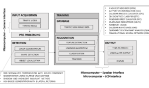
Figure 2: Overview of methodology

2.2        Pre-processing and Detection

The detection phase is composed of pre-processing, color-based segmentation, shape-based detection and object localization. This study will evaluate four different pre-processing and color-based segmentation methods that solved the problem of lighting variations affecting the detection phase. Methods to be evaluated that use different filtering techniques in different color spaces are RGB Normalized Thresholding with Color Constancy Algorithm, Segmentation using Relative Values of RGB, Shadow and Highlight Invariant Method, and HSV-based Segmentation with Bilateral Filtering.

2.2.1      RGB Normalized Thresholding with Color Constancy (CCM)

Histogram equalization of separate RGB channels is done followed by color constancy algorithm to extract the true color of the image [15]. The algorithm computes local space average color using a parallel grid of processing elements used to shift the color of the input pixel in the direction of the gray vector. Target color segmentation is done in HSV color space [16].

2.2.2       Segmentation using Relative Values of RGB (RRGB)

Segmentation that is based in three rules using the RGB color space. The pixel will be regarded as the target red color when (i) red component is greater than α, (ii) difference between red and green components is between β₁ and β₂ , and (iii) the difference between the red and blue components is between γ₁ and γ₂ . The values of α, β₁, β₂, γ₁, and γ₂ are experimentally found to represent the red color perceived in different lighting conditions [11].

2.2.3       Shadow and Highlight Invariant Method (SHI)

Utilized the normalized HSV color space values. Segmentation happens in the hue image where hue is 255 if the pixel’s hue is between 240 and 255, or hue is between 0 and 10. Hue will be set to 0 if pixel’s saturation is less than 40, or pixel’s value does not fall between 30 and 230. The hue image and seed image from the new hue is used, applying region growing algorithm to find target proper region [5].

2.2.4       HSV-based Segmentation with Bilateral Filtering (BFM)

Traffic images undergo pre-processing in the RGB color space before the detection stage. Bilateral filtering smoothens the image while preserving the edges by means of a nonlinear combination of nearby pixel values [24]. The weight assigned to each neighbor decreases with both the distance in the image plane and the distance on the intensity axis.

One of the four methods will be used for color-based segmentation to improve the efficiency and speed of detection of the next stage by reducing search areas that do not contain any possible traffic sign [9, 25] defined by pixels falling outside the target red color.

The next phase is the shape detection using Hough transform to detect the circular shape of the traffic sign. Hough transform has been recognized as a robust technique in curve detection that can detect objects even when polluted by noise [26]. It transforms a set of feature points in the image space into a set of accumulated votes in a parameter space. For each feature point, votes are accumulated in an accumulator array for all parameter combinations. Only one circle, by means of highest number of votes, will be detected as increasing the number of detection will also increase the time required to process multiple regions for the succeeding phases. The last stage in the detection phase is the object localization or the cropping of the candidate traffic sign from the traffic image to be used for the classification stage.

2.3        Feature Extraction

Histogram of Oriented Gradients (HOG) features are extracted from the candidate traffic sign images by the Python program to become the key feature for classification for the nine machine learning algorithms. The image from the dataset undergoes RGB to grayscale conversion and edge detection. The resulting image is then resized before using the built-in HOG extractor library in Python [6].

The steps above are important in ensuring optimum accuracy of the features when training the machine learning classifiers. HOG feature provides excellent performance relative to other existing feature sets [27].

2.4        Classifier

To classify the candidate traffic sign images, learning algorithms will be used. For this study, ten learning algorithms are implemented using sci-kit learn library [28] and Pytorch [29] in Python. The classifiers [30] to be evaluated based on accuracy and processing speed for traffic sign recognition are as follows.

2.4.1       K Nearest Neighbor (KNN)

KNN is a method where classification is computed from a simple majority vote of the nearest neighbors of each point [31]. Existing Python implementation of KNN uses model

KNeighborsClassifier(nneighbors=1) where a single neighbor is obtained for prediction.

2.4.2       Support Vector Machine (SVC)

An SVM is a discriminative classifier formally defined by a separating hyperplane. The algorithm outputs an optimal hyperplane using labeled training data which categorizes where the new examples are [32]. Implementation of the SVC will make use of the model SVC(kernel=”linear”,C=0.025) for linear kernel and with regularization parameter C of 0.025.

2.4.3       Gaussian Process Classifier (GPC)

Gaussian Processes predict by computing for empirical confidence interval using probabilistic Gaussian distribution [33]. For GPC implementation, the model GaussianProcessClassifier(1.0 * RBF(1.0)) will be used utilizing the default squared-exponential kernel as radial basis function.

2.4.4       Decision Tree Classifier (DTC)

Decision Trees are non-parametric supervised learning method used for classification and regression with goal of creating a model that predicts the value of a target variable by learning simple decision rules inferred from the data features [34]. The model to be used will be DecisionTreeClassifier(maxdepth=5) with maximum depth of the decision tree equal to 5. The deeper the tree, the more complex the if-then-else decision rules and the fitter the model.

2.4.5       Random Forest Classifier (RFC)

Random Forest algorithm is a supervised classification algorithm which creates a forest with a number of trees. The higher the number of trees in the forest gives the high accuracy results [35]. The model to be used is RandomForestClassifier(maxdepth=5, nestimators=10, maxfeatures=1) utilizing 10 decision trees, each with maximum depth of 5 and considering only 1 feature when looking for the best split.

2.4.6       Multilayer Perceptron (MLPC)

MLPC can be viewed as a logistic regression classifier where the input is first transformed using learnt non-linear transformation that projects the input data into a space where it becomes linearly separable [36]. Existing implementation model MLPClassifier (alpha=1e-5) will be used with L2 penalty parameter or regularization term equal to 0.00001. Smaller value of alpha may fix high bias which is a sign of underfitting by encouraging larger weights, potentially resulting in a more complicated decision boundary, while larger alpha value helps in avoiding overfitting by penalizing weights with large magnitudes [30]

2.4.7       AdaBoost (AdaB)

An AdaBoost classifier is a meta-estimator that begins by fitting a classifier on the original dataset and then fits additional copies of the classifier on the same dataset but where the weights of incorrectly classified instances are adjusted such that subsequent classifiers focus more on difficult cases [37]. The model AdaBoostClassifier() will be used utilizing default hyperparameter values where the base estimator is a decision tree classifier with a maximum depth of 1 and the maximum number of estimators is 50.

2.4.8       Gaussian Naive Bayes (GNB)

GNB is a special type of NB algorithm used when the features have continuous values and assumes that all the features are following a Gaussian distribution i.e, normal distribution. It scales cubically with the size of the dataset and might be considerably faster [38].

The model to be utilized calls GaussianNB().

2.4.9       Quadratic Discriminant Analysis (QDA)

QDA is closely related to LDA but uses quadratic decision surface. It can be derived from simple probabilistic model where prediction is obtained by using Bayes’ rule. The model fits a Gaussian density to each class [39]. In QDA, individual covariance matrix is estimated for every class of observations. QDA becomes useful when there is prior knowledge that individual classes exhibit distinct covariances. The model that will be utilized is QuadraticDiscriminantAnalysis().

2.4.10      Convolutional Neural Network (CNN)

It is a neural network mathematical model based on connected artificial neurons similar to biological neural networks. Neurons are organized in layers and connections are established between neurons of adjacent layers. The output layer neurons amount is equal

to the number of classifying classes with probabilities showing the possibility that the input vector belongs to a corresponding class [18]. The training process is to minimize the cost function with minimization methods based on the gradient decent also known as backpropagation [19]. The CNN model to be utilized is based on LeNet-5 architecture [40] composed of seven layer combination of convolution, pooling with rectified linear unit (ReLU) activation function and fully connected layers shown in Figure 3.

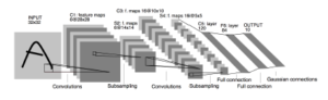
Figure 3: CNN model based on LeNet-5 architecture [40]

Table 1 summarizes the modification to hyper-parameter values done for the implementation of all the learning algorithms using scikit learn and Pytorch libraries in Python. All other hyper-parameters not modified are set to their default values.

Table 1: Summary of modified hyper-parameters for learning algorithms implementation

Learning Algorithm	Modified Hyper-parameter
KNN	n neighbors=1
SVC	kernel=”linear”, C=0.025
GPC	None
DTC	max depth=5
RFC	max depth=5, n estimators=10, max features=1
MLPC	alpha=1e-5
AdaB	None
GNB	None
QDA	None
CNN	6 classes output

2.5        Evaluation

The evaluation phase of the designed model will be divided into three: detection, recognition, and system level testing. For this study, the detection and recognition models will be tested individually based on accuracy and speed using Lenovo U410 ultrabook before a system level testing is performed.

2.5.1       Detection Model Testing

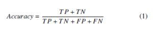
After implementation of the four pre-processing and segmentation models, traffic images will be fed. Accuracy will be computed using Equation 1. TP is defined by correct detection on image with traffic sign, TN when there is no detection for traffic image without traffic sign, FP for detection when the image has no traffic sign or detection of other part of the image with traffic sign, and FN for non-detection of the traffic image with traffic sign. Processing speed of the sub-processes will also be measured for the entire detection process.

2.5.2       Recognition Model Testing

For the testing of the implemented recognition model, cross validation method will be used wherein portion of the dataset will be used for training while the remaining will be for testing. A confusion matrix will then be generated. Evaluation metric to be used is accuracy that determines whether a label predicted for a sample exactly matches the corresponding true label of the sample. Equation 1 will be used to compute for accuracy. Processing time of the entire recognition model and its sub-processes will also be recorded.

2.5.3       System Level Testing

For the system level testing, the best detection and recognition models based on the evaluation will be integrated to create the entire model of the system using Nvidia Jetson Nano with interface Waveshare 7” LCD, IMX219-77 camera and generic speaker. Accuracy and speed of detection will be tested using an actual video taken in local road. System level accuracy will be computed to be the product of detection accuracy and recognition accuracy using Equation 1.

A successful recognition means that the system has provided a voice alert about the detected traffic sign. A text-to-speech python module will be used for this function and the corresponding voice alert for each traffic sign detected is shown in Table 2. A text annotation will also be generated to the display.

Table 2: Voice alert and text annotation for target traffic signs

Traffic Sign	Voice Alert	Text Annotation
Left Turn Prohibition	No Left Turn	No Left Turn
Right Turn Prohibition	No Right Turn	No Right Turn
U-Turn Prohibition	No U-Turn	No U-Turn
Overtaking Prohibition	No Overtaking	No Overtaking
30kph Speed Limit	Thirty kph	30 kph
60kph Speed Limit	Sixty kph	60 kph

3. Results and Analysis

3.1        Dataset

A total of 2,194 images are used to test the detection phase of the models. Of these, 2,170 are traffic images from online sources with traffic sign having different viewing angle and position on image. These are evenly distributed to the six traffic sign classes and an additional class for images without traffic sign with 1366×768 pixels resolution. The remaining 24 images with 1936×1296 pixels resolution are foreign traffic images captured at different distances from 10 meters to 120 meters with 10-meter increment. For the recognition models, 12,120 images will be used to evaluate speed and accuracy. This dataset is augmented using different cropping methods including zooming, north-west cropping and south-east cropping to act as learning compensation when segmentation of the traffic sign is not centered. The dataset will be divided into train data (10%, 5%, 1%) and test data (90%, 95%, 99%) to determine the effect of the number of test data to models’ accuracy. Another set contains six video footages with 360 frames of traffic images, 308 frames of which contain traffic sign. These are recorded using the actual system camera setup attached in a sedan car while approaching the traffic sign to be detected. Figure 4 shows a sample frame image from a video of a local road while Figure 5 shows sample images from the Napier University traffic dataset.

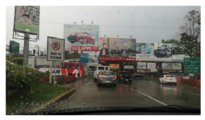
Figure 4: Sample traffic image from local road

Figure 6 shows the sample traffic signs from the dataset to be classified. This dataset contains a total of 2,020 images per class for the training and testing phases and is composed of different signs ranging from high resolution images up to 699×693 pixels down to low-resolution images of 12×12 pixels.

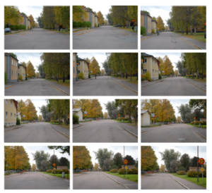
Figure 5: Sample traffic images from Napier University dataset

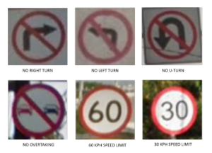
Figure 6: Sample traffic sign dataset

3.2        Traffic Sign Detection

The detection process is summarized by Figure 7 where the highlighted blocks are to be replaced by each of the four detection methods to be evaluated. From the original traffic image, red pixels are segmented using color thresholding. The resulting mask undergoes edge detection before Hough transform is applied to detect circular shape. The center and radius information is used to crop the candidate traffic sign for the next phase of classification. A traffic sign is considered detected if the cropped image fully shows the entirety of the traffic sign including the red circular boundary.

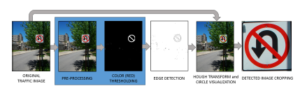
Figure 7: Traffic sign detection process

Experimentation for segmenting the red boundary of the traffic sign using HSV and relative RGB color spaces have resulted to the following threshold range summarized in Table 3 and Table 4. Figure 8 shows masks of segmented red color from an original traffic image using Relative RGB and HSV color segmentation.

Table 3: Range values for HSV color segmentation

Color Component/Channel	Range

Table 4: Range values for relative RGB color segmentation

Color Component/Channel	Range

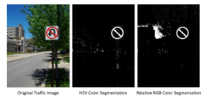
Figure 8: Sample relative RGB and HSV segmented red mask

Table 5: Accuracy of pre-processing and color segmentation methods

Method	Total Images	TP	TN	FP	FN	Accuracy
RRGB	2,170	535	299	11	1,462	32.12%
SHI	2,170	576	292	18	1,284	40.00%
BFM	2,170	503	304	6	1,357	37.19%
CCM	2,170	586	294	16	1,274	40.55%

Table 5 summarized the evaluation of the four pre-processing and color segmentation methods. In terms of accuracy, Color Constancy method provided the best performance successfully detecting 586 traffic signs from 2,170 traffic images. It is closely followed by the Shadow and Highlight Invariant method with 576 detection. Bilateral Filtering method and Color Constancy method have Shadow and Highlight Invariant method for color detection but results show improvement with Color Constancy method while performance degradation for Bilateral Filtering method due to (1) color improvement done by the Color Constancy method to the traffic image, and (2) images from the dataset are generally blurry due to vehicle vibration and environmental parameters that affect the performance of the Bilateral Filtering method. For Relative RGB implementation, color segmentation resulted to less false detection. Figure 9 shows the result of successful detection of traffic signs for six traffic images taken from local road using Shadow and Highlight Invariant method.

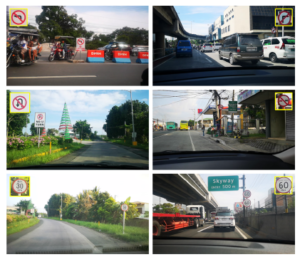
Figure 9: Sample detection of traffic sign

Table 6: Number of successful segmentation of pre-processing and color segmentation methods vs. traffic sign capturing distance

Distance	RRGB	SHI	BFM	CCM
120m	0	0	0	0
110m	0	0	0	0
100m	0	0	0	1
90m	0	0	0	0
80m	0	0	0	1
70m	0	2	1	1
60m	0	2	2	2
50m	0	2	2	2
40m	0	2	2	2
30m	0	2	2	2
20m	0	2	2	2
10m	2	2	2	2

Table 6 shows the evaluation of segmentation success of traffic sign with varying capturing distances. The traffic sign is captured twice per given distance. Color Constancy algorithm correctly segmented 15 out of 24 traffic images in the dataset with detection distance up to 100 meters. Shadow and Highlight Invariant Method correctly segmented 14 out of 24 images with detection distance up to 70 meters. Bilateral Filtering Method correctly detected 13 out of 24 images with detection distance up to 70 meters. Relative RGB Method has the worse performance detecting only 2 out of 24 images with detection distance up to 10 meters and false detecting 13 images. This result validates the accuracy evaluation of the four methods previously discussed in Table 5 and suggests that traffic sign distance affects the image feature clarity of the sign on the image and causes significant decrease in detection success rate.

Table 7 summarizes the processing speed of the four preprocessing and color segmentation methods including execution speed of their sub-processes. This timing does not include shape detection and ROI localization as these processes are common to all methods. Relative RGB segmentation has the fastest processing time closely followed by the Shadow & Highlight Invariant method. The slight difference is due to color space conversion from RGB to HSV. Different processor runtime caused variable timing result for color segmentation process for Shadow & Highlight Invariant, Bilateral Filtering, and Color Constancy. These two employed simple pre-processing while Color Constancy and Bilateral Filtering methods are pre-processing methods themselves and perform multiple and complex image filtering using kernels.

Considering accuracy and processing speed, the pre-processing and segmentation method that provided the best trade-off is Shadow and Highlight Invariant method with 40.00% segmentation success rate and 31.2 ms processing speed.

Table 7: Processing speed of pre-processing and color segmentation methods and sub-processes

Method	Pre-processing	Color Segmentation	Total
RRGB	10.4 ms	15.6 ms	26.0 ms
SHI	5.2 ms	26.0 ms	31.2 ms
BFM	270.8 ms	18.2 ms	289.0 ms
CCM	494.8 ms	20.8 ms	515.6 ms

3.3        Feature Extraction

HOG feature extraction of a traffic image is shown in Figure 10. It starts from grayscale conversion followed by edge detection then by HOG feature extraction. HOG feature represents the general structure of the image using the dominant orientation of pixel groups. This process transforms the 2D image into 1D vector histogram representing the gradient direction of the image.

3.4        Classifier Evaluation

Table 8 shows the result of implementation of traffic sign classification using Multi-layer Perceptron Classifier with variable image input resolution. This shows that more feature pixels will not always provide the best accuracy for a given classifier and the optimum image resolution considering accuracy and processing speed is 50×50 pixels.

Table 9 summarizes the result of evaluating the 10 classification algorithms in terms of accuracy with the number training data varied. Most of the model showed downward trend in accuracy when training data is decreased. GPC, though has one of the best accuracy for higher number of training data, provided the worse performance for decreasing training data since optimization is being done using squared-exponential kernel to best fit few training data leading to misclassification. Convolutional Neural Network implementation obtained the best accuracy among the models. This is due to learning optimization using backpropagation decreasing the loss function resulting to higher classification success rate. With lesser training data, CNN still has the best accuracy. This is important to consider to ensure that the model will still provide better accuracy even when trained with fewer data. Figure 11 shows the normalized confusion matrix generated for CNN classifier.

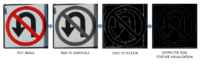
Figure 10: Test image feature extraction

Table 8: Effect of input image size to accuracy and processing speed for MLPC

Input Image Resolution	Accuracy	Processing Time
200×200 pixels	88.89%	454.5 ms
100×100 pixels	88.49%	331.2 ms
50×50 pixels	91.23%	283.2 ms
32x32pixels	85.32%	321.0 ms

Table 9: Effect of number of training data to accuracy

Classifier	10% Train	5% Train	1% Train	Average
KNN	94.63%	92.06%	86.70%	91.13%
SVM	89.72%	87.37%	57.21%	78.10%
GPC	93.87%	80.95%	16.63%	63.82%
DTC	72.45%	68.35%	57.90%	66.23%
RFC	76.59%	73.27%	60.17%	70.01%
MLPC	93.54%	91.19%	86.36%	90.36%
ADAB	62.50%	54.95%	35.64%	51.03%
GNB	85.44%	85.46%	77.50%	82.80%
QDA	54.07%	30.80%	26.28%	37.05%
CNN	96.64%	94.63%	87.64%	92.97%

K-Nearest Neighbor performed the second best in terms of accuracy closely followed by Multilayer Perceptron. This can be accounted to the characteristics of dataset. Each class of the dataset used is primarily composed of very similar images, and results suggest that KNN works better for data with close similarity.

The result of the evaluation of processing speed of the classification algorithms and their sub-processes for 90% of dataset is summarized in Table 10. CNN got the longest training time due to its nature of performing loss function optimization. Total recognition time is measured from color conversion until prediction and CNN obtained the fastest processing time. This is due to lesser pre-processing being implemented by the method unlike the other algorithms that still perform color conversion and extract HOG features to every input traffic sign image to classify. Recognition time for all classifiers is below 20 ms except for GPC with 750.6 ms due to the use of more complex squared-exponential kernel.

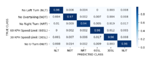
Figure 11: Normalized confusion matrix for CNN classifier

Table 10: Processing speed of classifiers and sub-processes

Classifier	Feature Extract	Train Time	Color Convert	Image Resize	Predict	TOTAL TIME
KNN	16.04s	0.05s	1.56ms	10.42ms	5.21ms	17.19ms
SVC	16.04s	0.64s	1.56ms	10.42ms	0.00ms	11.98ms
GPC	16.04s	272.8s	1.56ms	10.42ms	738.6ms	750.6ms
DTC	16.04s	0.47s	1.56ms	10.42ms	0.00ms	11.98ms
RFC	16.04s	0.02s	1.56ms	10.42ms	2.08ms	14.06ms
MLPC	16.04s	6.62s	1.56ms	10.42ms	0.00ms	11.98ms
AdaB	16.04s	5.32s	1.56ms	10.42ms	6.77ms	18.75ms
GNB	16.04s	0.03s	1.56ms	10.42ms	2.60ms	14.58ms
QDA	16.04s	0.43s	1.56ms	10.42ms	4.16ms	16.15ms
CNN	–	581.4s	–	5.21ms	2.60ms	7.81ms

Table 11 shows result of optimization of the best detection and classification models based on the evaluation. These models are Shadow and Highlight Invariant method and Convolutional Neural Network classifier.

Table 11: Optimization of detection and recognition models

Parameter	Original Model	First Optimization	Second Optimization
Total Images	2,170	2,170	2,170
TPdetection	576	1,372	1,372
TNdetection	292	300	300
FPdetection	18	40	40
FNdetection	1,284	458	458
TPrecognition	547	1,240	1,257
TNrecognition	NA	NA	4
FPrecognition	47	172	147
FNrecognition	NA	NA	4

The first optimization resulted to improvement of correct detection and significant decrease in false detection. The process involved modification of threshold parameters of Hough circle transform for it to detect circle less strictly since traffic sign boundaries most often are elliptical in shape in the traffic image due to variable viewing angle. Hough transform is also adjusted to only detect circles with diameter less than one fifth of the image height. The limiting of circular detection is important since detecting larger circles will result to more pixel features thus will require longer processing time. Also in actual application, traffic signs do not often occupy the entire traffic image.

For the second optimization where a seventh class is added, results in Table 11 show further increase in correct recognition and decrease in false recognition. The additional class filters signs that are similar to any of the six classes, and once recognized as false class, no output will be generated by the model.

Results show that the optimized integrated model has a detection performance of 77.05% and recognition performance of 89.31%. The relatively low detection performance is due to the failure of the Hough transform to detect the circular boundary of the traffic sign since the appearance of the traffic signs are affected by the viewing angle and effect of environmental setting to image quality. Although adjusting the detector threshold to lower value resulted to detection improvement, further decrease in threshold resulted to more false detection. The overall accuracy of the model is 68.81%.

3.5        System Implementation

After implementing the system using Nvidia Jetson Nano platform, a timing comparison between the performance of the system using Lenovo U410 Ultrabook is presented in Table 12. Training time and accuracy of both implementation are relatively the same. The huge difference lies in processing time with Nvidia Jetson Nano almost doubled that of the Lenovo U410. This is due to the clocking difference of the processors of the two platforms.

Table 12: Performance comparison between Lenovo U410 and Nvidia Jetson Nano

Parameter	Lenovo U410	Nvidia Jetson Nano
Training Time	678.94 s	679.10 s
Processing Speed	131.3 ms	238.0 ms
Accuracy	95.58%	97.24%

Figure 12 shows some of the successful detection and recognition where traffic signs are annotated to each frame of actual local road video. Table 13 summarizes the timing analysis of the entire TSDR system with text annotation and voice alert output. The system has a total processing time of 1.0953 seconds. It takes about 0.73 ms to display the text annotation of the detected and recognized traffic sign while it takes 938.21 ms for the system to utter the entire phrase for voice alert. For voice alert system, the next frame can only be processed after it has finished all the required processing for current frame including uttering the meaning of the sign.

Given this timing values, the system without voice alert and only using text annotation as output can run at a maximum frame rate of 1/116.7ms or approximately 8 frames per second. For the system with voice alert output, the system requires a frame rate of 1/1.0953 seconds or less than 1 frame per second for it to run in realtime. Since voice alert must be implemented, having a frame rate of less than 1 fps will result to poor sampling causing traffic signs to not be detected especially for fast moving vehicles. A solution is to implement adaptive frame rate such that during non-detection, the system will run at approximately 8 to 12 fps and when there is a traffic sign detected, frame rate shifts to approximately 1 fps to cater for the voice alert output. Figure 13 shows the hardware configuration block diagram of the system while Figure 14 shows the actual setup of the TSDR system for road testing. Figure 15 shows the testing of the TSDR system using actual footage from local road.

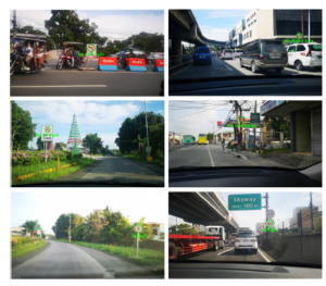
Figure 12: Sample detection and recognition of traffic frames

Table 13: Timing of sub-processes of the TSDR system

Process	Processing Time
Input Acquisition	13.69 ms
BGR to HSV Conversion	2.49 ms
Red Color Segmentation	5.22 ms
Gaussian Blurring	1.52 ms
Median Blurring	7.64 ms
Binary Thresholding	11.44 ms
Erosion	0.75 ms
Dilation	0.63 ms
Circle Detection	70.96 ms
ROI Cropping	7.09 ms
Image Transformation	4.79 ms
Prediction	30.13 ms
Text Annotation	0.73 ms
Voice Alert Output	938.21 ms
TOTAL TIME	1.0953 s

Table 14 shows the result of testing the TSDR system using a total of 360 frames from six different actual footage (F1-F6) from local roads. The footage contains 308 frames where traffic sign is fully visible with approaching distance and 52 frames where the traffic sign is not visible. The system had detection on 83 traffic images (TP_detection + FP_detection), of which 30 were classified correctly to not contain traffic signs (TN_recognition), 20 were correctly classified (TPrecognition), and 33 were incorrectly recognized (FPrecognition). The system has a detection accuracy of 32.50% and a recognition accuracy of 60.24%. The overall accuracy of the system is 19.58%. The low accuracy is due to the poor image quality caused by several factors including (1) poor camera, (2) vehicle motion and vibration, and (3) environmental setting.

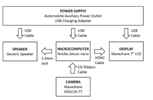
Figure 13: TSDR hardware configuration diagram

Detection and recognition of traffic sign in every frame is ideal for a ATSDR system but in actual application, one traffic sign correctly detected and recognized is enough to provide road information to the driver. Out of 6 sets of image sequences, 3 sets or 50% have at least one of the frames correctly detected and recognized.

Table 14: Test using frames from actual local road footage

Parameter	F1	F2	F3	F4	F5	F6	TOTAL
No. of Frames	87	73	64	32	48	56	360
TPdetection	12	29	2	0	0	23	66
TNdetection	12	7	8	8	8	8	51
FPdetection	3	8	0	0	0	6	17
FNdetection	60	29	54	24	40	19	226
TPrecognition	0	7	2	0	0	11	20
TNrecognition	9	15	0	0	0	6	30
FPrecognition	6	15	0	0	0	12	33
FNrecognition	0	0	0	0	0	0	0
Sign Detected?	No	Yes	Yes	No	No	Yes	50%

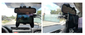
Figure 14: TSDR car setup for actual road testing

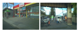
Figure 15: Sample frames from actual TSDR footage

4. Conclusion

Among the four evaluated pre-processing and detection methods, Shadow and Highlight Invariant method provided the best trade-off between segmentation success rate and processing time due to the less complex image filtering approach and use of HSV color space. Convolutional Neural Network classifier has the best performance in both accuracy and processing speed among the ten evaluated algorithms for traffic sign recognition due to the optimization method of the loss function using back propagation and the in-system feature extraction method of the algorithm. In classification, additional class to contain the not targeted traffic signs provides improvement of false detection performance.

An embedded system using Nvidia Jetson Nano platform with interface IMX219-77 camera, Waveshare 7” LCD and generic speaker using Python and OpenCV, sci-kit learn and Pytorch libraries has been developed. Implementation of adaptive frame rate improves sampling and provides an approach to handle variable frame processing time for a real-time system.

This study has not only provided comparative analysis on detection and recognition performance of several algorithms based on accuracy and processing speed but also able to implement a real-time embedded system. Further improvement to the system includes the use of better high definition camera with better image sensor and optical image stabilization. This can also be improved by the use of better detection and recognition algorithm like masked R-CNN. Also, further study can be done on the extension of application of the study to include other traffic signs and signals, and road markings.

Conflict of Interest

The authors declare no conflict of interest.

Acknowledgment

The authors would like to acknowledge Ateneo de Manila University, FAITH Colleges, and Fastech Synergy Philippines for supporting this research through their engineering scholarship program.

1. World Health Organization, “Global status report on road safety”, 2015, Re-trieved from
   https://www.who.int/violence injury prevention/road safety status/2015/en/
2. M. R. De Leon, “Towards Safer Roads: Road safety initiatives of DOTr”, ASEAN Automobile Safety Forum, May 2017.
3. A. C. Mendoza, “Applications of Psychology to the understanding and modifi- cation of road user behavior”, University of the Philippines National Center for Transportation Studies, August 2006.
4. Y. MaryReeja, T. Latha, A. MaryAnsalinShalini, “Traffic sign detection and recognition in driver support system for safety precaution”, ARPN J. Eng. Appl. Sci., 10, 2015, 2209-2213.
5. S. Feng, “Evaluation of colour segmentation algorithms in red colour of traffic sign detection”, M.S. Thesis, Department of Computer Engineering, Hogskolan Dalarna, 2010.
6. A. Santos, P. A. Abu, C. Oppus, R. Reyes, “Traffic sign detection and recogni- tion for assistive driving”, in 2019 International Symposium on Multimedia and Communication Technology (ISMAC), Quezon City, Philippines, 2019, pp. 1-6, doi: 10.1109/ISMAC.2019.8836161.
7. Department of Public Works and Highways, “Highway safety design standards, road safety design manual”, May 2012.
8. C. Mythili, V. Kavitha, “Color image segmentation using ERKFCM”, Int. J. Comput. Appl., 41(20), 21-28, March 2012, doi: 10.5120/5809-8074.
9. H. Fleyeh, M. Dougherty, “Road and traffic sign detection and recognition”, Advances OR and AI Methods in Transportation.
10. V. Deshmukh, G. Patnaik, and M. Patil, “Real-time traffic sign recognition system based on colour image segmentation”, 2013, Int. J. Comput. Appl., 83(3), 30-35, doi: 10.5120/14430-2575 10.5120/14430-2575.
11. C. Lin, C. Su, H. Huang, K. Fan, “Colour image segmentation in various illumination circumstances” in Proceedings of the 9th WSEAS International Conference on Circuits, Systems, Electronics, Control & Signal Processing. World Scientific and Engineering Academy and Society (WSEAS), Stevens Point, Wisconsin, USA, 2010, 179184, doi: 10.13140/2.1.1045.3446.
12. H. Rashmi, M. Shashidhar, G. Prashanth Kumar, “Automatic tracking of traf- fic signs based on HSV” International Journal of Engineering Research & Technology, 3(5), May 2014.
13. S. Sural, G. Qian, S. Pramanik, “Segmentation and histogram generation using the HSV color space for image retrieval” in Proceedings of the International Conference on Image Processing, Rochester, NY, USA, 2002, pp. II-II, doi: 10.1109/ICIP.2002.1040019.
14. H. Fleyeh, “Color detection and segmentation for road and traffic signs,” IEEE Conference on Cybernetics and Intelligent Systems, 2004, Singapore, 2004, pp. 809-814, doi: 10.1109/ICCIS.2004.1460692.
15. H. Fleyeh, “Traffic signs color detection and segmentation in poor light con- ditions”, MVA2005 IAPR Conference on Machine Vision Applications, May 16-18, 2005 Tsukuba Science City, Japan.
16. M. Ebner, “Color constancy using local color shifts”, The 8th European Conf. on Computer Vision, Prague, Czech Republic, 2004, 276-287, doi: 10.1007/978-3-540-24672-5 22.
17. H. Gomez-Moreno, S. Maldonado-Bascon, P. Gil-Jimenez, S. Lafuente- Arroyo, “Goal evaluation of segmentation algorithms for traffic sign recog- nition” in IEEE T. Intel. Transp., 11(4), pp. 917-930, Dec. 2010, doi: 10.1109/TITS.2010.2054084.
18. A. Shustanov, P. Yakimov, “CNN design for real-time traffic sign recognition”, Procedia Eng., 201, 718-725, 2017, doi: 10.1016/j.proeng.2017.09.594.
19. S. Prasomphan, T. Tathong, P. Charoenprateepkit, “Traffic sign detection for panoramic images using convolution neural network technique”, HPCCT 2019: Proceedings of the 2019 3rd High Performance Computing and Cluster Tech- nologies Conference, 2019, 128-133, doi: 10.1145/3341069.3341090.
20. Y. Wu, Y. Liu, J. Li, H. Liu, X. Hu, “Traffic sign detection based on convolu- tional neural networks”, Proceedings of the International Joint Conference on Neural Networks, 2013, 1-7, doi: 10.1109/IJCNN.2013.6706811.
21. Y. Sun, P. Ge, D. Liu, “Traffic sign detection and recognition based on convolu- tional neural network,” 2019 Chinese Automation Congress (CAC), Hangzhou, China, 2019, pp. 2851-2854, doi: 10.1109/CAC48633.2019.8997240.
22. D. Alghmgham, G. Latif, J. Alghazo, L. Alzubaidi, “Autonomous traf- fic sign (ATSR) detection and recognition using deep CNN”, Pro- cedia Comput. Sci., , 2019, Pages 266-274, ISSN 1877-0509, https://doi.org/10.1016 2.108.
23. D. Tabernik, D. Skoaj, “Deep learning for large-scale traffic recognition” IEEE T. Intel. Transp., 21(4), pp. 1427-1440, April 2020, doi: 10.1109/TITS.2019.2913588.
24. C. Tomasi, R. Manduchi, “Bilateral filtering for gray and color images,” Sixth International Conference on Computer Vision (IEEE Cat. No.98CH36271), Bombay, India, 1998, pp. 839-846, doi: 10.1109/ICCV.1998.710815.
25. N. Kehtarnavaz, A. Ahmad, “Traffic sign recognition in noisy outdoor scenes,” Proceedings of the Intelligent Vehicles ’95. Symposium, Detroit, MI, USA, 1995, pp. 460-465, doi: 10.1109/IVS.1995.528325.
26. M. Rizon, H. Yazid, P. Saad, A. Shakaff, A. Saad, “Object detection using circular hough transform”, American Journal of Applied Sciences, 2, 2005, 10.3844/ajassp.2005.1606.1609.
27. N. Dalal, B. Triggs, “Histograms of oriented gradients for human detection,” 2005 IEEE Computer Society Conference on Computer Vision and Pattern Recognition (CVPR’05), 1, San Diego, CA, USA, 2005, pp. 886-893, doi: 10.1109/CVPR.2005.177.
28. J. Lim, C. Oppus, “Identifying car logos using different classifiers in Python with HOG features”.
29. A. Paszke, S. Gross, F. Massa, A. Lerer, J. Bradbury, G. Chanan, T. Killeen, Z. Lin, N. Gimelshein, L. Antiga, A. Desmaison, A. Kopf, E. Yang, Z. DeVito,
30. Raison, A. Tejani, S. Chilamkurthy, B. Steiner, L. Fang, J. Bai, S. Chintala, “PyTorch: An imperative style, high-performance deep learning library”, Adv. Neur. In., 32, 2019.
31. F. Pedregosa, G. Varoquaux, A. Gramfort, V. Michel, B. Thirion, O. Grisel,  Blondel, P. Prettenhofer, R. Weiss, V. Dubourg, J. Vanderplas, A. Passos, uchesnay, “Scikit-learn: machine learning in python”, J. Mach. Learn. Res. 12, pp. 2825-2830, 2011.
32. Nearest Neighbors Classification. Retrieved from https://scikit- learn.org/stable/modules/neighbors.html
33. Introduction to Support Vector Machines. Retrieved from https://docs.opencv.org/3.4/d1/d73/tutorial introduction to svm.html
34. Gaussian Processes. Retrieved from https://scikit- learn.org/stable/modules/gaussian process.html
35. Decision Trees. Retrieved from https://scikit-learn.org/stable/modules/tree.html
36. How the Random Forest Algorithhm Works in Machine Learning. Retrieved from https://dataaspirant.com/2017/05/22/random-forest-algorithm-machine- learing/
37. Multilayer Perceptron. Retrieved from http://deeplearning.net/tutorial/mlp.html
38.  An AdaBoost Classifier. Retrieved from https://scikit-learn.org/stable/ mod- ules/generated/sklearn.ensemble.AdaBoostClassifier.html
39. Gaussian Nave Bayes Classifier Implementation in Python. Retrieved from https://dataaspirant.com/2017/02/20/gaussian-naive-bayes-classifier- implementation-python/ Linear and Quadratic Discriminant Analysis. Retrieved from https://scikit- learn.org/stable/modules/lda qda.html
40. Y. Lecun, L. Bottou, Y. Bengio, P. Haffner, “Gradient-based learning applied to document recognition,” in P. IEEE, 86(11), pp. 2278-2324, Nov. 1998, doi: 10.1109 1.

(Click Here)

(Click Here)