1. Introduction

The Hausdorff distance (HD) is an useful parameter for measuring the degree of resemblance between two point sets. The advantage of HD is that there is no requirement of point-to-point correspondence. In many science and engineering fields, HD has particular attention of researcher, such as face recognition [1–5], image matching [6–8], image segmentation for medical image [9–11], image retrieval [12,13], shape matching [14–16].

The HD is defined as MAX-MIN distance between two point sets, measuring how far two point sets are from each other. The HD computing contains two loops, the outer loop for maximization and the inner loop for minimization. Due to the sensitivity of the MAX-MIN HD with the outlier, average Hausdorff distance or partial Hausdorff distance (PHD) is used instead MAX-MIN HD in image matching or face recognition applications. Huttenlocher et al. The PHD was first proposed [17] for comparing the similarity between two shapes. In [18], the robust Hausdorff distance for face recognition was proposed, which uses PHD for measuring the distance between two sets of feature of face gray images. However, PHD is just an effective distance when the pollution of noise points is low. In face recognition research, average Hausdorff distance is commonly used.

The modified Hausdorff distance (MHD) was first presented [19] for image matching, where the directed Hausdorff distance is the mean of all distance from points to other sets. The ’doubly’ modified Hausdorff distance (M2HD), which is the improved of the MHD, was proposed for face recognition [20]. Various algorithms using average weighted HD, an extension of MHD, were proposed for face recognition with the difference in weighted function., i.e., spatially weighted Hausdorff distance (SWHD) [21], spatially weighted modified Hausdorff distance (SW2HD) [22], spatially eigen-weighted Hausdorff distances (SEWHD) [23], edge eigenface weighted Hausdorff distance (EEWHD) [24,25].

The extension of M2HD, similarity measure based on Hausdorff distance (SMBHD), was proposed for face recognition [3]. Another version of MHD, called modified Hausdorff distance with normalized gradient (MHDNG), was proposed for face recognition [8]. A new modified Hausdorff distance (MMHD) was presented for face recognition [26], which used average weighted Hausdorff distance for measuring the dissimilarity between two sets of dominant points of edge maps of face images. Based on edge map of face image, a novel face feature representation was proposed [27], line segment edge map (LEM). The line segment Hausdorff distance (LHD), which is the average weighted of distances between two line segments, was proposed for face recognition. Based on LHD, the extension of LHD, called spatial weighted line segment Hausdorff distance (SWLHD), was presented for face recognition [28] . In our previous work [1], we proposed a modification of LHD for face recognition, called Robust Line Hausdorff distance RLHD.

Supporting P and Q are the number of points, or elements, in two sets. For computing the directed distance of average HD, the distances from each point in the first set to all points in the second set have to be calculated to find the minimum value, which is the distance from the point in first set to its nearest neighbor in second set. The directed distance of average HD is the mean of all distances from points in first set to their nearest neighbors in second set. The computational complexities of methods using average HD are always O(PQ), the same as MAX-MIN HD. In recent decades, many methods have been proposed for reducing the computational complexity of the HD computing, which is known very high. The key of reducing the computational complexity is reducing the average number of the inner loop. All of these methods uses a temporary HD cmax for quickly finding the non-contributed points in the inner loops and outer loops for final HD computing. However, the these methods, which is proposed with the purpose of reducing the running time of MAX-MIN HD computing, can not be used for reducing computing complexity the average HD computing because the temporary HD cmax does not exist in average HD computing. Due to the high computing complexity of average HD, the face recognition methods, which use average HD for measuring the distance between two sets of feature, are restricted from face recognition applications.

Here we propose an extension of the method in [1], called Least trimmed square Line Hausdorff distance (LTS-LHD) for face recognition. The LTS-LHD, an extension of weighted average HD, is used for measuring the dissimilarity between two line edge maps (LEMs). The LTS-LHD is the average of largest distances instead of all distances as average HD. The experimental results shows that the face recognition accuracy of the proposed method, LTSLHD, is equivalent to the accuracy of LHD method, which used average HD for measuring distance between two LEMs, with a suitable parameter. Moreover, with LTS-LHD, the temporary HD cmax exist, and the methods, which are proposed with the purpose reducing the computational complexity of MAX-MIN HD computing, could be used for reducing the runtime of the proposed method. The EARLYBREAK [29], which is known as the stateof-art algorithm for reducing the computational complexity of HD computing, is used for reducing the computational complexity of proposed method. The runtime of proposed method is 68% lower than the LHD method.

The rest of the paper is structured as follows. The brief review of methods, which were proposed for reducing the computational complexity of the HD, is presented in Section 2. Section 3 presents the proposed method for face recognition, which uses LTS-LHD for measuring the distance between two LEMs. Section 3 also presents how to apply EARLYBREAK method for reducing the computational complexity of proposed method. Section 4 evaluates the performance of the proposed method and the performance of proposed method is also compared with the performance of LHD and RLHD method. Finally, conclusion is presented in Section 5.

2. Related works

Given two nonempty point sets M = ⁿm₁,m₂,…,m_p^o and T = ⁿt₁,t₂,…,t_q^o, the directed Hausdorff distance h(M,T) between M and T is the maximum distance of a point m ∈ M to its nearest neighbor t ∈ T. The directed Hausdorff distance from M to T as a mathematical formula is

where k.,.k is any norm distance metric, e.g. the Euclidean distance. Note that, in general case, h(M,T) , h(T, M) and thus directed Hausdorff distance is not symmetric. The Hausdorff distance between M and T is defined as the maximum of both directed Hausdorff distance and thus it is symmetric. The Hausdorff distance H (M,T) is defined as

With two point sets M and T, if the Hausdorff distance between

M and T is small, two point sets are partially matched, and if the Hausdorff distance is zero, two point sets are exactly matched.

Computing HD is challenging because its characteristics contain both maximization and minimization. Many efficient algorithms, in recent decades, have been proposed for reducing the computational complexity of the HD. We refer reader to the survey [17,30] for general overview of this field. The efficient computing HD algorithms can be generally divided into two categories, approximate HD and exact HD. In the first category, which is approximation of HD, the algorithms try to efficiently find an approximation of the Hausdorff distance. These algorithms have been widely used in runtime-critical applications. On the other hand, the algorithms of the second category aim to efficiently compute the exact HD for point sets or special types of point sets like polygonal models or special curves and surfaces. Depending on data type of two sets, the HD algorithms can also be classified as polygonal models, curves and mesh surfaces, point sets.

With data type is polygonal models, a linear time algorithm for computing HD between two non-intersecting convex polygons was presented in [31]. The algorithm has a computational complexity of O(m + n), where m and n are the vertex counts. In [32], an algorithm for computing the precise HD between two polygonal meshes with the complexity of On⁴ logn was presented. Due to the high computational complexity of exact HD calculation, approximate HD methods have been proposed. In [14], a method, that has the complexity of O (m + n)log(m + n), used Voronoi diagram to approximate the HD between simple polygons was presented. Another method for approximating the HD between complicated polygonal models was presented in [33]. By using Voronoi subdivision combined with cross-culling, non-contributing polygon pairs for HD are discarded. The method is very fast in practice and can reach interactive speed.

Many efficient algorithms were also proposed for calculating HD between mesh surfaces or curves. An efficient algorithm for calculating HD between mesh surfaces was presented in [34]. This algorithm is built on the specific characteristics of mesh surfaces, where the surface consists of triangles. To avoid sampling all points in the compared surfaces, the algorithm samples in the regions where the maximum distance is expected. The method for calculating the HD between points and freeform curves was presented in [35]. In [36], the improved method of [35] was presented for computing HD between two B-spline curves. For approximating the HD between curves, in [37], an algorithm was proposed, that converts the problem of computing HD between curves to the problem of computing distance between grids. In [38], an algorithm to compute the approximate HD between curves was presented. By approximating curves with polylines, the problem of computing HD between curves is converted to the problem of computing HD distance between line segments.

However, above methods are not general because the algorithms are based on specific characteristic of data types. Some general methods were proposed for point sets. An algorithm for finding the aggregate nearest neighbor (ANN) in database was proposed [39], that uses the R-Tree for optimizing the searching for ANN. The extension of [39], incremental Hausdorff distance (IHD) was proposed in [40] for efficiently calculating HD between two point sets. The algorithm uses two R-Trees for the same time, each for one point set, to avoid the interaction of all points in both sets. The aggregate nearest neighbor is simultaneously determined in both directions. However, complex structure of above algorithms makes the computation cost increase and the R-Tree is not suitable for general point sets.

In [29], a fast and efficient algorithm for computing exact Hausdorff distance between two point sets, which is known as a state-ofart algorithm, was proposed. The algorithm has two loops, with the outer loop for maximization and the inner loop for minimization. The inner loop can break as soon as the distance is found that is below the temporary HD (called cmax) because the rest iterations of inner loop do not make the value of cmax change, and the outer loop continues with the next point. Moreover, for improving performance, random sampling is also presented in this algorithm to avoid similar distances in successive iterations. Based on EARLYBREAK [29], an efficient algorithm, namely local start search (LSS) or Z-order Hausdorff distance (ZHD), for computing exact HD between two arbitrary point sets was presented [41]. The LSS method uses Morton curve for ordering points. The main idea of the LSS algorithm is that if the break occurs in current loop at the point x, it is quite possible that the break will occur at the position near x in the next loop. In the LSS algorithm, the variable preindex is used for preserving the location of break occurrence. In the next outer loop, the inner loop starts from preindex and scan its neighbor for finding the distance below the value cmax. In [42], an efficient framework, which contains two sub-algorithms Non-overlap Hausdorff Distance (NOHD) and Overlap Hausdorff Distance (OHD), for computing the HD between two general 3D point sets was proposed. For 3D point sets, [43] presented diffusion search of efficient and accurate HD computation between 3D models. This proposed method contains two algorithms for two types of 3D model, the ZHD for sparse point sets and the OHD for dense point sets.

In this study, we proposed the Least Trimmed Square Line Hausdorff Distance (LTS-LHD) for measuring the dissimilarity between two line edge maps (LEMs), which are the sets of line segments. The Hausdorff distance between two point set is based on the spatial locality of two point sets. Thus, the structure R-Tree of ANN and IHD or Z-order of LSS are just suitable for ordering the point sets [41]. However, the Hausdorff distance between two sets of line segments is based on both the spatial locality and the direction of line segment. Therefore, the structure R-Tree of ANN and IHD or Z-order of LSS are not suitable for the set of line segments as LEM, and thereby, the EARLYBREAK is used for reducing the complexity of computing the LTS-LHD.

3. Proposed method

3.1        LTS-LHD for face recognition

The original HD, the MAX-MIN distance, uses the distance of most mismatched points for measuring the distance between two sets. When the set is attacked with noise points, the original HD can not be used. The PHD was proposed for solving this problem by sorting the distance and taking the K ranked maximum value. However, PHD is an effective distance when the pollution of noise points is low. The MHD was also proposed for solving the problem of sensitivity of original HD with noise by taking the mean distance. As in [44], the LTS-HD was proposed for combining the advantage of the PHD and the MHD. The definition of directed LTS-HD from M to T is as follow

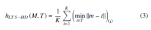
where the (minkm − tk)_(i) represents the i^th distance in the sorted sequence (minkm − tk)_m∈M. The LTS-HD takes the mean of K minimum distances for measuring the distance between two sets.

In this paper, a new HD, called Least Trimmed Square Line Hausdorff Distance (LTS-LHD), for face recognition is proposed.

Supporting M^l = ⁿm^l₁,m^l₂,..,m^l_P^o and T^l = ⁿt₁^l ,t₂^l ,..,t_Q^{l o} are the LEMs of model and test images respectively; m^l and t^l are the line segments in the LEMs; P and Q are the number of line segments in model and test LEMs, respectively. The directed distance of the

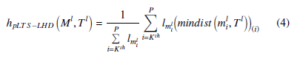
LTS-LHD from LEM M^l to LEM T^l, h_pLTS−LHD M^l,T^l, is defined

^Pth lm_li i=Kth i=K

where mindist m^l_i,T^l_(i) presents the i^th value in the sorted sequence in ascending order mindist m^l,T^l ; and K^th = f ∗P,

(m_l∈M_l)

 ^l,T^l denotes the diswhere f is a given fraction. The mindist m_i tance from the line segment m^l to its nearest neighbor in T^l, and it is defined as below

where d m^l,t^t is the distance between two line segments m^l and t^l. Here, the directed distance of the LTS-LHD is used for measuring how far from LEM M^l to LEM T^l. So, different from the LTS-HD as in (3), where the directed distance is the average of smallest distances, the distance as in (4) is the weighted average of largest distances, which are greater or equal to the K^th ranked value, from line segment m^l to its nearest neighbor mindist m^l,T^l. However, the directed distance of the LTS-LHD as in (4) still has weakness. Supporting m^l₁ and m^l₂ are two line segments in M^l, d₁ and d₂ are two distances from these segments to their neighbors. Assuming d₁ is greater than the K^th ranked value and d₂ is less than the K^th ranked value of the sorted sequence mindist m^l_i,T^l_(ml_∈Ml₎. As in (4), d₁ is used for the computing of h_pLTS−LHD M^l,T^l. However, it is possible that l_ml1.d₁  l_ml2.d₂, because line segment m^l₂ is much longer than line segment m^l₁. The miss match of the long line segment is more serious than the short line segment. So, the line segment m^l₂ is much more important than the line segment m^l₁ for computing the directed distance of LTS-LHD. Here, we modify the (4) for proposing the directed distance of the LTS-LHD as follow

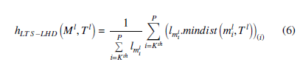
where l_mli .mindist m^l_i,T^l_(i) presents the i^th value in the sorted sequence in ascending order l_ml .mindist m^l,T^l(m_l∈Ml₎. The directed distance of the LTS-LHD is the weighted average of largest values of the product between length of line segment and the distance from that line segment to its nearest neighbor l_ml .mindist m^l,T^l.

In general, hLTS−LHD Ml,Tl , hLTS−LHD Tl, Ml. Thus, the primary LTS-LHD is defined as

In our previous work [1], a new data structure of LEM was proposed. Due to the angle between line segments and the horizontal axis, the line segments in LEM are grouped into N groups and

180/N degrees for each group. For example, in this paper, we use N = 18. An example of new data structure of LEM is shown in Fig1.

The distance between two line segments d m^l,t^l is defined as

where V is the value that is larger than the largest possible value

  ^l − t^l    is the distance of distance between two line segments;   m between two line segments and defined as

where d_pa is the parallel distance, which is the vertical distance

between two lines; d_pe is the perpendicular distance, which is minimum displacement to align either the left end points or the right end points of two lines; and d_θ m^l_i,t^l_j = θ² m^l_i,t^l_j/W is the orientation distance. θ² m^l_i,t^l_j is the smallest intersection angle between two lines and W is a weight, which could be determined by a training process.

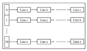
Figure 1: A novel data structure for LEM

It is possible that the line segment m^l could take a line t^l, that intersection angle between m^l and t^l is large, as it nearest neighbor. However, the line segment reflects the structure of human face, two corresponding line segments can not have large angle variation. For alleviating the undesire mismatch, the line segment finds its nearest neighbor if the group index (g_ml and g_tl ) of two line segments are slightly different as in (8). On the other hand, the distance between two line segments takes a large value V.

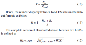
The number of corresponding line pairs between the model and the test LEM can be used as other measure similarity. Because test and model images are aligned and scaled at the same size by preprocessing before matching, if the line segment m^l finds that line segment t^l is the nearest neighbor in T^l and line segment t^l locates in the position neighborhood N_p of m^l, such line segment m^l could be named as high confident line. A high confident ratio, as in [27], of an image could be defined as the ratio between number of high confident line segments (N_hc) and number of total line segments in the LEM of face image (N_total) as follow

where W_n is a weight that be determined by a training process.

3.2        EARLYBREAK for LTS-LHD

The directed distance of the LTS-LHD as in (6) is the weighted average of P − K^th largest values of the product between length of line segment and distance to its nearest neighbor l_ml .mindist m^l,T^l. For computing the directed distance of the LTS-LHD, the distances from line segment m^l to all of line segments in T^l must be calculated for finding the minimum value, which is the distance from line segment m^l to its nearest neighbor mindist m^l,T^l. This process could be named as the inner loop. The inner loop must be performed with all line segments m^l ∈ M^l and we call this is the outer loop. Assuming that P − K^th temporary largest values are found and the minimum of these values is assigned to cmax. If a line segment m^l in the outer loop find out a line segment t^l in inner loop that makes the product between length of line segment m^l and distance d m^l,t^l between two line segments is below the value of cmax, such line segment m^l is non-contributed line segment for the computing of the directed distance LTS-LHD. So, the computing distance from line segment m^l to the remaining line segments t^l is not necessary. Therefore, the computing of directed distance LTS-LHD could break and continuing with the next line segment in the outer loop as soon as a non-contributed line segment be found. Thus, the number of iterations of the inner loop is reduced. The lower of average number of inner iteration is, the lower of computational complexity of the LTS-LHD computing is. Here, we proposed a method using EARLYBREAK for reducing the computational complexity of the LTS-LHD by reducing the average number of inner iterations.

The Algorithm 1 describes our proposed method. Line 5 and line 13 are the outer loop and the inner loop, respectively. The function DIST (.,.) in the Algorithm 1 is used for calculating the distance between two line segments as in (9).

The main steps of the Algorithm 1 are summarized as follows:

• A matrix h is created for saving the length of line segment m^l and the value of the product between length of line segment m^l and distance to its nearest neighbor.
• Adding line segments t^l having group index g_t into list.
• If there is at least one line segment in list, the inner loop will be executed. For each line segment m^l ∈ M^l, initializing distance to nearest neighbor cmin = ∞.
  • For each line segment in list, the distance from m^l to t^l is calculated. If a distance makes the product between it and length of line segment below the value of cmax, the algorithm will break and continue with the next

line segment in the outer loop. In the other hand, this distance is used for updating the value of cmin.

• The product between cmin and length of line segment will be used for updating the matrix h.

• On the other hand, if there is no line segment in list, the matrix h will be updated with length of line segment m^l and the large value V, which is the distance from line segment m^l to its nearest neighbor.
• The matrix h will be sorted in ascending order for each interaction of outer loop according to the values of the first row of matrix h.

In the Algorithm 1, during first K_M iterations of the outer loop, the value of cmax, which is the minimum value of matrix h, is 0.

The condition as line 15 in the Algorithm 1 does not appear, thus, the early break does not occur in first K_M iterations of the outer loop. The first K_M iterations of the outer loop, the value of K_M elements in the matrix h are updated. In the next iterations of the outer loop, the early break occurs if the value of product between the length of line and its distance to the nearest neighbor is below cmax.

Algorithm 1 : EARLYBREAKING for LTS-LHD

1: Inputs: Edge map Ml and Tl, fraction f   2: Outputs: Directed Hausdorff distance hLTS−LHD Ml,Tl 3: KM = (1 − f) ∗ P 4: h = zeros(2, KM) 5: for each line segment ml in edge map Ml do
6:	cmax = h(1,1)
7:	Get the group index gm of line segment ml
8:	cmin = ∞
9:	for gt = gm − k : gm + k do
10:	Insert line segments tl has group index gt into list
11:	end for
12:	if list is not empty then
13:	for each line segment tl in list do
14:	d = DIST ml,tl
15:	if d ∗ lM ≤ cmax then
16:	cmin = 0
17:	break
18:	end if
19:	if cmin > d then
20:	cmin = d
21:	end if
22:	end for
23:	if (cmin ∗ lM) > cmax then
24:	h(1,1) = cmin ∗ lM
25:	h(2,1) = lM
26:	end if
27:	else
28:	h(1,1) = V ∗ lM
29:	h(2,1) = lM
30:	end if
31:	sort h in ascending order of the value of first row
32: end for hLTS−LHD Ml,Tl = sum(h(1,:))/sum(h(2,:)) 33:

By using the face database of Bern university [45] for training process, we obtain that: W = 45, Np = 6 and Wn = 13.

3.3        Analysis of computational complexity

Supporting P and Q are the number of line segments in LEM M^l and in LEM T^l, respectively. In the LHD method [27], each line segment m^l ∈ M^l calculate the distance to all line segments in T^l for finding its nearest neighbor. The directed distance of the LHD is the weighted average of the distances from line segments m^l ∈ M^l to their nearest neighbors in T^l. So, the complexity of computing directed distance of the LHD is O(PQ).

The directed distance LTS-LHD computing as in (6) has computational complexity O(PQ) in the worst case. In the worst case, all of line segments of two LEMs are located in the same group, and each line segment has to calculate distance to all line segments in other LEMs for finding nearest neighbor. On the other hand, with the best case, if all line segments of each LEM are located in one group and two groups of two LEMs are much different, the computational complexity of directed Hausdorff distance is O(P). If the line segments of LEM T^l are equally divided into 18 groups, the computational complexity of directed Hausdorff distance would be O(PQ(2k + 1)/N), where k is the difference of group index as defined in (8). The computational complexity of the LTS-LHD is always better than the LHD because the lower bound of the LTS-LHD computational complexity is the LHD computational complexity.

The Algorithm 1, in which the EARLYBREAK is applied for the LTS-LHD, has the computational complexities O(P) and O(PQ) for the best case and the worst case, respectively. In general case, assuming that line segments of LEM are equally divided into groups, the Algorithm 1 has a computational complexity of O((1 − f) PQ(2k + 1)/N + fPX), where X is used to denote the average number of iterations in the inner loop. The lower value of X is, the lower of computational complexity of the method is and vise versa. The question is, in general, how high of the value of X is? In the formal way, the value of X in general case could be found through the analysis of probability theory.

Considering picking a random line segment t^l in the inner loop of the Algorithm 1, the distance d measured between line segment t^l and line segment m^l in current outer loop is a random variable. The event that meeting the condition that d is over cmax is denoted as e. The probability of that event is that P(e) = q. The event e means non-appearance of the break in the algorithm. Obviously, the event e, that d is less than cmax, occur with probability P(e) = p = 1 − q.

Assuming that the inner loop has been implemented for X times before the break occurs. This is equivalent to that (X − 1) distances from line segment m^l in the outer loop to the line segments t₁^l ,t₂^l ,…,t_X^l ₋₁, namely d₁,d₂,…,d_X−1, are over cmax and one distance d_X ≤ cmax. The probability density function of X is given by

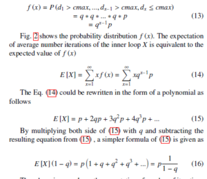
Then, by using p = 1−q, the expectation of number of iterations in the inner loop X could be found as

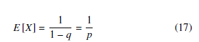
Equation (17) means that the number of iterations in the inner loop until the break depends on the value of p, which is the probability that a distance d is less than cmax. The higher p means the lower number of tries before early break and vice versa. The value of p depends on the value of cmax. For a larger value of cmax, it is easier for picking a line segment making the distance d to the current line segment of the outer loop less than cmax. Fig. 3 illustrates the relation between cmax and the probability p. Here, it is assumed the distance d is a random variable with normal distribution for illustration. The value of p does not depend on the size of set, but rather on the value of cmax and the distribution of pairwise distance d.

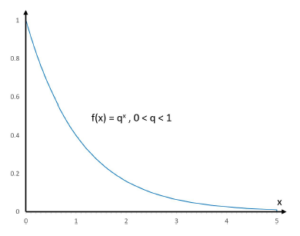
Figure 2: Probability density function f (x)

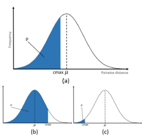
Figure 3: Normal distribution of pairwise distance is assumed. (a) Relation between cmax and probability p. (b) Large value of cmax. (c) Small value of cmax.

4. Experiments

In this section, the performance of the proposed method, LTS-LHD, is evaluated for face recognition. It is done by measuring the distance from test image to all model images for finding the smallest distance. The recognition rate, which is the ratio of number of images correctly classified to the total number of images in the test set, is used for evaluating.

In this study, the face database from the University of Bern [45] and the AR face database from Purdue University [46] are used. Bern university face database contains frontal views of 30 people. Each person has 10 gray images with different head pose variations: two frontal pose images, two looking to the right images, two looking to the left images, two looking upward image and two looking downward images. The AR face database contains 2599 color face images of 100 people (50 men and 50 women), there are 26 images for each person and be divided into 2 sessions separated by two weeks interval. Each session has 13 images are the frontal view faces with different facial expressions, illumination conditions, and occlusions (sun glasses and scarf). However, one of frontal face image is corrupted (W-027-14.bmp) and only 99 pairs of face image are used for examining the performance of system for face recognition under normal conditions. In our experiment, a preprocessing before recognition process is used for locating the face. All image are normalized such that the two eyes were aligned roughly at the same position with a distance of 80 pixels. After that, all images are cropped with size 160 × 160 pixels. The experiments are conducted on the PC with 3GHz CPU and 4GHz RAM.

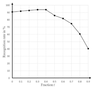
Figure 4: Influence of fraction f on recognition rate for AR database

4.1        Influence of fraction f on the performance

The recognition rate of the proposed method is expected to be low for both low and high values of fraction f. With high value of fraction f, a low number of line segments, which have largest values of the product between their length and distance to their neighbor, is used for computing the directed distance of the LTS-LHD. However, the outliers are commonly the line segments have largest values of that product. The high value of f means most of line segments used for computing the directed distance LTS-LHD are outliers, as in (6). On the other hand, when the value of fraction f is too low, a high number of line segments is used for computing the directed distance of the LTS-LHD. This means high number of line segments in similar regions of faces is used for the calculation of h_LTS−LHD. And thus, the contribution of line segments that discriminate the faces becomes low.

Fig. 5 shows the recognition rate of the proposed method for the

AR database with various values of fraction f. It must be noticed that the value f of 1 is meaningless, because the value of directed distance of the LTS-LHD h_LTS−LHD is zero for all face image pairs. The proposed method has highest recognition rate at the fraction f values 0.3 and 0.4.

The computational complexity of the proposed method is based on the average number of iterations in the inner loop, and thus is based on the value of cmax. The higher value of cmax is, the lower of runtime is and vice versa. The low value of fraction f means the large number of line segments is used for computing h_LTS−LHD, and the value of cmax becomes low. On the other hand, the high value of fraction f means the high value of cmax, and thus the computational complexity of the method is low. So, the value of fraction f is chosen at 0.4.

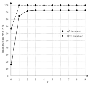
Figure 5: Influence of parameter k on recognition rate of proposed method

4.2        Influence of parameter k on the performance

The recognition rate of the proposed method is expected to be low for low value of parameter k and vice versa. As in algorithm 1, the value of k determines the number of line segments in the inner loop. The low value of k has strong effect on system performance. Supporting m^l is the line segment in current outer loop. The low value of k means m^l has to find its nearest neighbor in a few number of line segments in list, as in algorithm 1. And thus it is possible that list does not contain the corresponding line segment of m^l, and m^l could take another non-corresponding line segment as its nearest neighbor. On the other hand, the higher value of k is not necessary because too much line segments, which are too far from m^l, are added into list. Such non-contributed line segments make the number of iterations of inner loop increase and thus the runtime of method increases. Fig. 5 shows the recognition rates of the proposed method with various values of k for both the Bern university database and the AR database. The recognition rate does not change for the value of k higher than 2 for the Bern university database and 3 for the AR database. So, the chosen value of k is 3.

In the rest of this section, the recognition rate of the proposed method is compared with the LHD method in [27] and the RLHD method in [1], using average HD for measuring the dissimilarity between LEMs.

4.3        Face recognition under normal conditions

The frontal face images in normal conditions in the Bern university database and the AR database are used for evaluating the performance of the proposed method. Each person has two images, one for test set and one for the model set. The example of images in this experiment is shown in Fig. 6. The recognition rates of different methods are given in Table. 1. The recognition rates of all methods with Bern university database are higher than those with the AR database. The reason is the different between two images of each person in AR database is larger than Bern database. The illumination of model image and test image in AR database are also different. The recognition rate of the proposed method is equal to the RLHD method.

• Bern University Database
• AR Database

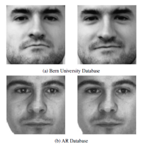
Figure 6: Example of two pairs frontal face image in normal lighting condition in the face database of Bern University and the AR face database

Table 1: Face recognition result

	Recognition rate
Method	Bern database	AR database
LHD	100%	93%
RLHD	100%	94%
Proposed method	100%	94%

The matching time for the Bern university database of different methods are given in Table. 2. The proposed method has the runtime 68% lower than the LHD method and 17.5% lower than RLHD method. The improvement in runtime is achieved by using EARLYBREAK for reducing the average number of iterations in the inner loop.

Table 2: Matching time of different methods

Method	LHD	RLHD	Proposed method
Matching time (second)	337	131	108

4.4        Face recognition under varying lighting conditions and poses

The performance of the proposed method is also compared with the ones of the LHD and the RLHD methods for face recognition in the non-ideal conditions, e.g. face image with different poses or different lighting conditions. The AR database is used for evaluating the performance of different methods with varying lighting conditions of face image. Frontal face images of 100 people are used as model set. The face images with a light source on left side of face, with a light source on right side of face and with light sources on both sides of face are divided into three test sets with 100 images for each set. The recognition rates of different methods are given in Table. 3. The non-ideal lighting conditions make the recognition rate of all methods approximate 10% decrease. The face recognition accuracy of proposed method is 1%, on average, higher than the LHD and the RLHD methods. The interesting point of the experiment is that all three methods, in the condition of left light on, give the same recognition rates as the normal lighting condition in Table. 1 while the recognition rate in right light on condition is 6% – 9% lower than the ideal lighting condition. This could be due to the fact that the illumination of the right light is stronger than the left light. When both light on, the recognition rates of all methods are 12% lower than recognition rates in ideal lighting condition. The over-illumination has strong effect on recognition rates of all methods.

Table 3: Face recognition with varying lighting conditions

Lighting conditions	LHD	RLHD	Proposed method
Left light on	93%	94%	94%
Right light on	87%	85%	88%
Both light on	71%	72%	72%
Average	83.67%	83.67%	84.67%

The Bern university database is used for evaluating the performance of different methods with different poses of face image. The model set contains 30 frontal face images of 30 people. The test set contains images of 30 people with different poses, e.g. looking to the left and right, looking up and down, for each person. The recognition rates of different methods are summarized in Table. 4. The pose variations have strong effect on recognition rates of all methods, where the recognition rates decrease 40% – 50% in comparing with the results in Table. 1. This could be explained that there are portions of face missing in comparing with frontal face. The recognition rate of the proposed method is lower than the RLHD method with the looking right image and higher than the RLHD methood in other conditions. On average, the proposed method has the recognition rate 2% higher than the RLHD method and 3% higher than the LHD method.

Table 4: Face recognition with varying poses

	LHD	RLHD	Proposed method
Looking left	46.67%	53.33%	63.33%
Looking right	53.33%	46.67%	46.67%
Looking up	66.67%	63.33%	66.67%
Looking right	60%	70%	63.33%
Average rate	56.67%	58.33%	60%

5. Conclusion

The Hausdorff distance, which is used for measuring the degree of resemblance between two geometric objects, has been widely used in various science and engineering fields. The computational of HD computing is high because the computing contain both maximization and minimization. Many methods have been proposed in recent decades for reducing the computational complexity of MAXMIN HD computing. However, the proposed methods for reducing the computational complexity of MAX-MIN HD computing can not be used for reducing the computational complexity of average HD computing. In face recognition, average HD is widely used for measuring the distance between two sets of features, instead of MAX-MIN HD, which is known as a sensitive measure with noise. The computational complexity of average HD computing as high as the MAX-MIN HD computing. The high computational cost restricts face methods using he average HD from real time applications.

The LHD and he RLHD use average HDfor measuring the dissimilarity between two LEMs. In this paper, a modification of RLHD, called LTS-LHD was proposed for face recognition. The LTS-LHD uses only K_M line segments, not all of line segments as in RLHD, for calculating the directed distance. With a suitable parameter K_M, or suitable fraction f, the proposed method, LTS-LHD, has the performance slightly higher than the RLHD method, which is the average HD.

Moreover, in this paper, the EARLYBREAK is used for reducing the computational complexity of the proposed method. The early breaking can speed up the LTS-LHD by reducing the average number of iterations in the inner loop. The experimental results show that the runtime of proposed method is 68% lower than the LHD method and 17.5% lower than the RLHD method.

Acknowledgment

We acknowledge the support of time and facilities from Ho Chi Minh City University of Technology (HCMUT), VNU-HCM for this study.

1. C. Dang-Nguyen, T. Do-Hong, “Robust line hausdorff distance for face recognition, in 2019 International Symposium on Electrical and Electronics Engineering (ISEE), HoChiMinh, Vietnam, 2019. https://doi.org/10.1109/ISEE2.2019.8921218
2. J. Wang and Y. Tan, “Hausdorff distance with k-nearest neighbors, in Proceedings of the Third International Conference on Advances in Swarm Intelligence – Volume Part II, ser. ICSI12. Berlin, Germany, 2012. https://doi.org/10.1007/978-3-642-31020-1
3. Y. Hu, Z. Wang, “A similarity measure based on hausdorff distance for hu- man face recognition, in 18th International Conference on Pattern Recognition (ICPR’06), Hong Kong, China, 2006. https://doi.org/10.1109/ICPR.2006.174
4. S. Chen and B. C. Lovell, “Feature space hausdorff distance for face recognition, in Proceedings of the 2010 20th International Conference on Pattern Recogni- tion (ICPR’10), Istanbul, Turkey, 2010. https://doi.org/10.1109/ICPR.2010.362
5.  J. Paumard, “Robust comparison of binary images,” Pattern Recognition Letters, 18(10), 1057 1063, 1997. https://doi.org/10.1016/S0167-8655(97)80002-5
6. H. Zhu, T. Zhang, L. Yan, and L. Deng, “Robust and fast haus- dorff distance for image matching,” Optical Engineering, 51(1), 2012. https://doi.org/10.1117/1.OE.51.1.017203
7. X. Li, Y. Jia, F. Wang, and Y. Chen, “Image matching algorithm based on an improved hausdorff distance,” in 2nd International Symposium on Com- puter, Communication, Control and Automation (3CA 2013) , Singapore, 2013. https://doi.org/10.2991/3ca-13.2013.61
8. C.H. Yang, S.H. Lai, and L.W. Chang, “Hybrid image matching combining hausdorff distance with normalized gradient matching,” Pattern Recognition, 40(4), 11731181, 2007. https://doi.org/10.1016/j.patcog.2006.09.014
9. D. Karimi and S. E. Salcudean, “Reducing the hausdorff distance in medical image segmentation with convolutional neural networks,” IEEE Transactions on Medical Imaging, 39(2), 499513, 2020. https://doi.org/10.1109/TMI.2019.2930068
10. H. Yu, F. Hu, Y. Pan, and X. Chen, “An efficient similarity-based level set model for medical image segmentation,” Journal of Advanced Me- chanical Design, Systems, and Manufacturing, 10(8), 01000108, 2016. https://doi.org/10.1299/jamdsm.2016jamdsm0100
11. F. Morain-Nicolier, S. Lebonvallet, E. Baudrier, S. Ruan, “Hausdorff distance based 3d quantification of brain tumor evolution from mri images,” 2007 29th Annual International Conference of the IEEE Engineering in Medicine and Biology Society, Lyon, 2007. https://doi.org/10.1109/IEMBS.2007.4353615
12. M. Grana, M. A. Veganzones, “An endmember-based distance for content based hyperspectral image retrieval,” Pattern Recognition, 45(9), 3472-3489, 2012. https://doi.org/10.1016/j.patcog.2012.03.015
13. Y. Gao, M. Wang, R. Ji, X. Wu, Q. Dai, “3-D object retrieval with hausdorff dis- tance learning,” IEEE Transactions on Industrial Electronics, 61(4), 20882098, 2014. https://doi.org/10.1109/TIE.2013.2262760
14. ] H. Alt, B. Behrends, J. Blomer, “Approximate matching of polygonal shapes,” Annals of Mathematics and Artificial Intelligence, 13, 251265, 1995. https://doi.org/10.1007/BF01530830
15. L. B. Kara and T. F. Stahovich, “An image-based, trainable symbol recog- nizer for hand-drawn sketches,” Computer Graphics, 29(4), 501517, 2005. https://doi.org/10.1016/j.cag.2005.05.004
16. M. Field, S. Valentine, J. Linsey, and T. Hammond, “Sketch recognition algo- rithms for comparing complex and unpredictable shapes,” in Proceedings of the Twenty-Second International Joint Conference on Artificial Intelligence – Volume Three (IJCAI ’11), Barcelona, Spain, 2011.
17. D. P. Huttenlocher, G. A. Klanderman, W. J. Rucklidge, “Comparing images using the hausdorff distance,” IEEE Transactions on Pattern Analysis and Machine Intelligence, 15(9), 850863, 1993. https://doi.org/10.1109/34.232073
18. V. E. P and N. Sudha, “Robust hausdorff distance measure for face recognition,” Pattern Recognition, 40(2), 431442, 2007. https://doi.org/10.1016/j.patcog.2006.04.019
19. M. P. Dubuisson and A. K. Jain, “A modified hausdorff distance for object matching,” in Proceeding 12th International Conference on Pattern recognition, Jerusalem, Israel, 1994. https://doi.org/10.1109 6361
20. B. Takcs, “Comparing face images using the modified hausdorff distance,” Pattern Recognition, 31(12), 18731881, 1998. https://doi.org/10.1016/S0031- 3203(98)00076-4
21. B. Guo, K. Lam, W. Siu, S. Yang, “Human face recognition using a spa- tially weighted hausdorff distance, in The 2001 IEEE International Sym- posium on Circuits and Systems (ISCAS 2001), Sydney, Australia, 2001. https://doi.org/10.1109/ISCAS.2001.921027
22. K. Lin, B. Guo, K. Lam, W. Siu, “Human face recognition using a spatially weighted modified hausdorff distance,” in Proceedings of 2001 International Symposium on Intelligent Multimedia, Video and Speech Processing. (ISIMP 2001), Hong Kong, China, 2001. https://doi.org/10.1109/ISIMP.2001.925437
23. K.H. Lin, K.M. Lam, and W.C. Siu, “Spatially eigen-weighted hausdorff dis- tances for human face recognition,” Pattern Recognition, 36(8), 1827 – 1834, 2003. https://doi.org/10.1016/S0031-3203(03)00011-6
24. H. Tan and Y. Zhang, “Computing eigenface from edge images for face recognition based on hausdorff distance,” in Fourth International Con- ference on Image and Graphics (ICIG 2007), Sichuan, China, 2007. https://doi.org/10.1109/ICIG.2007.70
25. H. Tan, Y.-J. Zhang, W. Wang, G. Feng, H. Xiong, J. Zhang, and Y. Li, “Edge eigenface weighted hausdorff distance for face recognition,” Interna- tional Journal of Computational Intelligence Systems, 4(6), 1422-1429, 2011. https://doi.org/10.1080/18756891.2011.9727894
26. Y. Gao, “Efficiently comparing face images using a modified hausdorff dis- tance,” IEE Procceeding Vision, Image and Signal Processing, 150(6), 346350, 2003. https://doi.org/10.1049/ip-vis:20030805
27. Y. Gao and M. K. H. Leung, “Face recognition using line edge map,” IEEE Trans. on Pattern Analysic and Machine Intelligence, 24(6), 764779, 2002. https://doi.org/10.1109/TPAMI.2002.1008383
28. C. Du, G. Su, X. Lin, “Face recognition using a modified line segment haus- dorff distance,” in Proceedings of the 2003 International Conference on Ma- chine Learning and Cybernetics (IEEE Cat. No.03EX693), Xi’an, China, 2003. https://doi.org/10.1109/ICMLC.2003.1260095
29. A. A. Taha and A. Hanbury, “An efficient algorithm for calculating the exact hausdorff distance,” IEEE Transactions on Pattern Analysis and Machine Intelli- gence, 37(11), 21532163, 2015. https://doi.org/10.1109/TPAMI.2015.2408351
30. H. Alt and L. J. Guibas, “Discrete geometric shapes: Matching, interpolation, and approximation, Handbook of computational geometry,” Elsevier, 2000.
31. M. J. Atallah, “A linear time algorithm for the hausdorff distance between convex polygons,” Information Processing Letters, 17(4), 207-209, 1983. https://doi.org/10.1016/0020-0190(83)90042-X
32. M. Barton, I. Hanniel, G. Elber, and M.-S. Kim, “Precise hausdorff distance computation between polygonal meshes,” Computer Aided Geometric Design, 27(8), 580-591, 2010. https://doi.org/10.1016/j.cagd.2010.04.004
33. M. Tang, M. Lee, Y. J. Kim, “Interactive hausdorff distance computation for general polygonal models,” ACM Transactions on Graphics, 28(3), 2009. https://doi.org/10.1145/1531326.1531380
34. M. Guthe, P. Borodin, R. Klein, “Fast and accurate hausdorff distance calcula- tion between meshes.” Journal of WSCG, 13(2), 41-48, 2005.
35. H. Alt and L. Scharf, “Computing the hausdorff distance between curved ob- jects.” International Journal of Computational Geometry and Applications, 18(4), 307320, 2008. https://doi.org/10.1142/S0218195908002647
36. X.D. Chen, W. Ma, G. Xu, and J.-C. Paul, “Computing the hausdorff distance between two b-spline curves,” Computer-Aided Design, 42(12), 1197 1206, 2010. https://doi.org/10.1016/j.cad.2010.06.009
37. E. Belogay, C. Cabrelli, U. Molter, R. Shonkwiler, “Calculating the hausdorff distance between curves.” Information Processing Letters, 64(1), pp. 1722, 1997. https://doi.org/10.1016/S0020-0190(97)00140-3
38. Y.B. Bai, J.H. Yong, C.Y. Liu, X.M. Liu, and Y. Meng, “Polyline approach for approximating hausdorff distance between planar free-form curves,” Computer-Aided Design, 43(6), 687698, 2011. https://doi.org/10.1016/j.cad.2011.02.008
39. D. Papadias, Y. Tao, K. Mouratidis, and C. Hui, “Aggregate nearest neighbor queries in spatial databases,” ACM Transactions on Database Systems, 30(2), 529576, 2005. https://doi.org/10.1145/1071610.1071616
40. S. Nutanong, E. H. Jacox, and H. Samet, “An incremental hausdorff distance calculation algorithm,” Proceedings of the VLDB Endowment , 4(8), 506517, 2011. https://doi.org/10.14778/2002974.2002978
41. Y. Chen, F. He, Y. Wu, and N. Hou, “A local start search algorithm to compute exact hausdorff distance for arbitrary point sets,” Pattern Recognition, 67, 139 148, 2017. https://doi.org/10.1016/j.patcog.2017.02.013
42. D. Zhang, F. He, S. Han, L. Zou, Y. Wu, and Y. Chen, “An effi- cient approach to directly compute the exact hausdorff distance for 3d point sets,” Integrated Computer-Aided Engineering, 24(3), 261277, 2017. https://doi.org/10.3233/ICA-170544
43. D. Zhang, L. Zou, Y. Chen, and F. He, “Efficient and accurate hausdorff dis- tance computation based on diffusion search,” IEEE Access, 6, 13501361, 2018. https://doi.org/10.1109/ACCESS.2017.2778745
44. G. Chen, Q. Dai, X. Tang, and Z. Xu, “An improved least trimmed square hausdorff distance finger vein recognition,” in 2018 5th International Conference on Systems and Informatics (ICSAI), Nanjing, China, 2018. https://doi.org/10.1109/ICSAI.2018.8599439
45. Bern University Database. http://www.fki.inf.unibe.ch/databases/iam-faces- database/FullFaces.tgz
46. A. Martinez and R. Benavente, “The AR face database,” CVC Technical Report, 24, Jun 1998.

(Click Here)

(Click Here)