1. Introduction

A firewall is an indispensable system for today’s computer networks. It plays an important role to prevent access to various resources on the networks, for example, networking devices, databases, web servers and etc. Besides, it can also prevent attacks and intrusions by malicious users from dark side networks. Basically, the firewall is commanded by a set of instructions, called the rule. The number of firewall rules depends on the complexity of the policies of each organization. As the number of rules increases, the number of anomaly rules is also enlarged. The anomalies arise from two or more rules overlapping but having different decisions. There are five types defined by [1]: the shadowing, correlation, generalization, redundancy, and irrelevancy anomaly. Recently, a new definition of anomalies has been advanced, which is the semantics loss of rules [2]. The rule anomalies have a great impact on the overall performance of a firewall. That is, they decrease the processing speed of rule verifying or matching. Therefore, reducing the number of anomalies improves the speed of the rule verification as well. Analyzing, managing and resolving anomalies are big problems of firewall researches and attract much interest. The first major researcher about the anomalies was Al-Shaer, who presented five types of anomaly rules and also invented an effective method for detecting anomalies, called the finite state diagram [3]. Later, several researchers contributed various methods for detecting anomalies, for example, in [4] the authors revealed a powerful algorithm to relieve the root cause of anomalies, called SDD. However, the rules are only one type either “an acceptable status” or “an unacceptable status” appearing on the firewall. Next, in [5] they proposed a method to resolve the anomaly problems effectively by using the firewall decision diagram (FDD) and this is also the prototype of much other later research. The propositional logic model was presented by [6], they claimed that their model could remove anomalies that lead to a decrease in the number of rules without changing the policy. Next, in [7] authors demonstrated the anomaly management framework which encourages systematic detection and resolution of firewall policy anomalies based on the average risk values, called FAME. The risk values are calculated from the Common Vulnerability Scoring System (CVSS) [8] which does not consider attacking vulnerabilities in the overview, but it is considered only the point. The next proposed solution for analyzing and managing the firewall policies was Lumeta [9] and Fang [10]. They represented the tools that are used to analyze firewall rules, but tools cannot completely verify the misconfigurations policy settings. In [11] the authors contributed an algorithm for detecting and resolving conflicts in packet filtering. Though, the algorithm can only detect certain specific conflicts. The firewall rule optimization based on Service-Grouping was proposed by [12]. The basis of this technique is resolving the conflicts segment by grouping rules from work behaviors. They claimed that the processing time and number of packet hits are better than the traditional and FIREMAN [13] firewall. FPQE [14] is an automated system to resolve rule anomalies, which does not require any admin intervention. It uses an automatic rule removal in the case of redundancy and contradiction anomaly, and uses an automatic rule permutation against shadowing and correlation. Besides, some techniques allow the firewall to automatically detect and analyze conflict rules such as [15] and [16], but they are not based on real tangible evidence. By most methods, the burden of resolving rule conflicts is often given to the administrator’s discretion instead.
This paper contributes the model for optimizing firewall rule anomalies by applying the probability (Bayesian) together with evidence of each rule, i.e., frequency of packets matching against rules, evidence of creating rules, the expertise of rules and protocol priority. This model provides guidance to firewall administrators to resolve rule anomalies with probability values. In order for administrators to be confident that the decision is more accurate based on the actual evidence. This paper is organized as follows: Section 2 overviews the background and related work. Section 3 presents the key contributions. In Section 4 articulates our system design. Section 5 addresses the implementation of details and evaluations. Section 6 concludes this paper.

Background and Related Works

Rule Definition and Anomaly
Generally, the firewall rule consists of two parts: the condition and decision parts. Let R be a firewall rule, C as a condition part and A is a decision part, a firewall rule format:

In fact, firewalls always have more than a single rule. Therefore, the first equation (1) needs to be revised to the second equation:

where C_i and A_i are the condition and decision of rule R_i (Any firewall rule) by i∈[1,n], and n is a non-negative integer. Given f_i representing the domain of positive integers is a finite range, denoted 〖D(f〗_i). For example, the domain of the source and destination address in an IP packet is [0, 232 – 1] (〖D(f〗_1) and 〖D(f〗_2)), source and destination port is [0, 216 – 1] (〖D(f〗_3) and 〖D(f〗_4)) and protocol is [0, 28 – 1] (〖D(f〗_5)). C_i defines a set of packet fields over the fields f_1 through f_d specified as f_1∈F_1∧f_2∈F_2∧…〖∧f〗_d∈F_d where F_i is a subset of 〖D(f〗_i). A_i is either accept or deny for each rule. If all conditions (f_i) in C_i are true, the decision is either accept or deny depending on the specified administrators like:
R_1=〖〖(f〗_1∧ f_2∧f_3∧…∧ f_d)〗_1→〖accept〗_1 |〖deny〗_1
Given P_i as an IP packet over the d fields f_1, …, f_d, P_i is a tuple of 〖d(p〗_1, p_2, …, p_d) where each p_i (1≤i≤d) is an element of 〖D(f〗_i). An IP packet 〖(p〗_1, p_2, …, p_d) matches R_i if and only if the condition p_1∈f_1∧p_2∈f_2∧…〖∧p〗_d∈f_d. A set of rules 〖(R〗_1,…,R_i) is valid when there is at least one rule in the set matching against p_i. To make sure that firewall rules are working properly, the condition of the final rule in the firewall is usually specified as f_1∈D(f_1 )∧…〖∧f〗_d∈D(f_d), where every packet must be matched as shown in R_3, called the implicit rule. The set of rules below shows an example of three rules over the three fields of condition 〖C(f_1,f_2,f_3)〗_i where 〖D(f〗_1)= D(f_2 )∈[1,100] and 〖D(f〗_3)∈[1,50].
R_1=〖(f〗_1∈[25,50]∧ f_2∈[40,60]∧f_3∈[5,25])→accept
R_2=〖(f〗_1∈[35,70]∧ f_2∈[30,90]∧f_3∈[10,25])→accept
R_3=〖(f〗_1∈[1,100]∧ f_2∈[1,100]∧f_3∈[1,50])→deny
R_1 and R_2 are redundant because any packet can match both rules which have the same actions (accept). Furthermore, R_1 and R_2 also conflict with R_3 because both R_1 and R_2 are subsets of R_3 while they are different actions. One typical solution to resolve such conflicts, that is, firewalls choose a rule which matches with the packet p_i being considered first, called the first-match approach. The firewall rules anomalies can be classified into six [1], [2] types representing each anomaly by the theorems:
Shadow anomaly: R_x is shadowed by R_y, if and only if their intersection is equal to R_x and there are different actions illustrated in Figure 1(a).

where R_db is a database of all rules, and R_y is the rule executed before R_x.
Correlation anomaly: R_x and R_y in R_db are correlated if their intersection is not equal to ∅, R_x-R_y≠∅,R_y-R_x≠∅, and they have different actions represented in Figure 1(b).

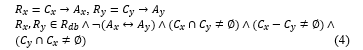
where R_db is a database of all rules, and R_y is the rule executed before R_x.
Generalization anomaly: R_x is generalized by R_y, if and only if their intersection is equal to R_y, and there are different actions (Figure 1(c)), where R_y is the rule matched before

Redundancy anomaly: R_x is redundant to R_y, if and only if their intersection is not equal to ∅, and they are have same actions (Figure 1(d)).

Irrelevance anomaly: Irrelevance anomaly occurs in the firewall if no packets can be matched against all rules in the firewall. This anomaly is caused by the administrator’s misunderstanding about the network connections.

where P_i is an IP packet executed by the firewall.
Semantics loss anomaly: The semantics loss represented by [2] occurs when R_x and R_y are merged to R_z by the meaning of both old rules that have been changed or replaced by a new meaning. This anomaly is mostly caused by redundant rules as shown in Figure 1(f).

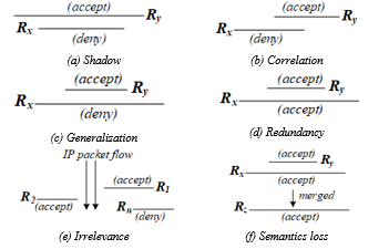Figure 1: Firewall rule anomalies

Min-Max Feature Scaling

Min-Max feature scaling [17] (also known as data normalization) is the standard method used to adjust the range of data. Since the range of data values may be very different, it is therefore a necessary step in data preprocessing before processing in the next step. It is normally used to resize any data range into the range [0, 1], called unity-based normalization. Also, it can normalize the finite range of values in the dataset between any arbitrary points t_max and t_min as the following equation.

Let m^’ denotes the value being considered has been normalized by m ∈[r_min,r_max]. r_min and r_max denote the minimum and maximum of the measurement range. t_minand t_max are the minimum and maximum of the target range to be scaled.

Bayes’ Theorem

Bayes’ theorem [18] (also known as Bayes’ rule) is a formula that describes how to update the probabilities of hypotheses when given evidence. It is a useful tool for calculating conditional probabilities. Bayes’ theorem can be defined as follows.
Let A_1,A_2,〖…,A〗_k be events that partition the sample space S, i.e., S= A_1∪A_2∪…∪A_k and A_i∩A_j≠∅ when i≠j and let B be an event on that space for which P_r (B)>0. Then Bayes’ theorem is:

This formula can be used to reverse conditional probabilities. If we know the probabilities of the events A_j and the conditional probabilities P_r (〖B|A〗_j), j=1,…,k, the formula can be used to compute the conditional probabilities P_r (A_j│B).

Moving Average (MA)

A moving average (MA) [17] is a widely used indicator for analyzing data trends. It helps smooth out data action by filtering out the disturbance from short-term data fluctuations. There are two types of basic moving averages, which are popular and widely used, namely Simple Moving Average (SMA) and Exponential Moving Average (EMA). SMA calculates an average of the last n data, where n represents the number of periods for which we need the average.

where A_i is an average in period n, and n is the number of periods. EMA is a weighted average of the last n data, where the weighting decreases exponentially with each previous data per period. In other words, the formula gives greater weight to more recent data. The formula for the exponential moving average is the following.

where 〖EMA〗_t = EMA today, V_t = Value today, 〖EMA〗_y = EMA yesterday, s = smoothing, d is the number of day.

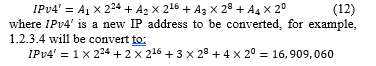
Converting an IP Address to a non-negative Integer

The Internet Protocol Address (as known as IP Address) is a unique address that networking devices such as routers, switching, and computers use to identify themselves and communicate over other devices in computer networks. An IPv4 address (IP version 4) is equal to 32 bits, ranging from 0 to 232 – 1 address space. It is usually divided into four parts, each part (8 bits = an octet) separated by a dot, e.g., A_1.A_2.A_3.A_4 where A_((1 – 4))∈[0,255]. IPv4 address can be converted to any non-negative integer with the following equation.

Arithmetic Mean and Kappa Statistics
We use the average method (x ̅ ) to evaluate the administrator’s satisfaction with the proposed firewall and use the Cohen’s kappa coefficient ((K_F ) ̂) [19] to measure the interrater reliability as the following equations.

where x ̅ is an average (or arithmetic mean), n is the number of terms (e.g., the number of items or numbers being averaged), and x_i is the value of each individual item in the list of numbers being averaged.

where: P ̅_a denotes the relative observed agreement among raters, P ̅_e denotes the hypothetical probability of chance agreement as in the equation 15 and 16.

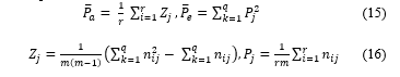
where m is the number of raters, the objective of the assessment is r, q is the type of information that needs to be evaluated (e.g., most satisfied, very satisfied, …, least satisfied), and n_ij denotes the observed cell frequencies.

Key Contributions

As rule anomalies occur over firewalls, the decision-making power to resolve the anomalies mainly depends on the administrator’s discretion. However, the decisions made often result in errors or loopholes over the existing rules, if admins cannot entirely understand the relationship between conflict rules. Therefore, it is necessary to develop a decision support system for admins to assist decision-making during real-time anomaly detection. The system consists of four procedures:
Firstly, preparing various information to be ready before processing,
Analyzing and detecting the rule abnormalities by the Path Selection Tree (PST),
Calculating the probability (Bayesian) of each rule based on the frequency of packets matched against rules, evidence of creating rules, expertise on creating rules, and protocol priority to help admins decide before optimizing the rules,
Lastly, optimizing anomaly or conflict rules based on the probability.

The System Design

There are four steps in the system design as shown in Figure 2.
Preparing Rule-Based Firewall (Step 1)
The conditions (C_i) and decision (A_i) of each rule: Referring to R_i in the equation (2), in general, the members of C_i have five fields (f_1 ∧ … ∧ f_5), where f_1 = source IP address (SIP), f_2 = destination IP address (DIP), f_3= source port (SP), f_4 = destination port (DP) and f_5 = protocol (PRO) respectively as shown in Table 1. According to R_1 of Table 1, the preparation process of firewall rules begins with converting the IP addresses of f_1 and f_2 into a range of positive integers by equation (12). Hence, f_1 and f_2 are then converted into the following numbers: f_1 ∈ [16909056, 16909066] and f_2 ∈ [1, 256]. The fields converted in the next order are f_3 and f_4 which contain the numbers ranging from 0 to 216 – 1: f_3 ∈ [0, 65535] and f_4 ∈ [80, 80], where ∗ means all numbers in such domain. The field f_5 is both TCP and UDP protocol, thus they are translated to: f_5 ∈ {6, 17}, where TCP = 6 and UDP = 17. In case of decision field (A_i), it is changed to a positive integer either 0 or 1, such as A_i ∈ {0, 1}, where accept = 1 and deny = 0. As a result of all these calculations, R_1 is converted to:

R_1:(f_1∈[16909056,16909066]∧f_2∈[1,256]∧f_3∈
[0,65535]∧f_4∈[80,80]∧f_5∈{6,17})→1
Table 1: The basic member fields of C_i and A_i

Ri	Ci(f1˄ f2˄ f3˄ f4˄ f5)					Ai
R1	f1(SIP)	f2(DIP)	f3(SP)	f4(DP)	f5(PRO)	decision
R1’	1.2.3.0- 1.2.3.10	0.0.0.1- 0.0.1.0	*	80	TCP, UDP	accept

Calculating Probability of Extra Fields of Each rule: To determine the probability of each rule in this model, there are four additional fields added including the frequency of packets matching against rules (FPM), evidence of creating rules (ECR), the expertise of rules creator (ERC) and protocol priority (PRI). Let P(e_1), P(e_2), P(e_3) and P(e_4) are the probability of FPM, ECR, ERC, and PRI respectively. Therefore, the sum of the probability of rule R_i is equal to the equation (17).

Where P(E_i ) is the probability of R_i. For example, the information of extra fields of R_i as shown in Table 2. From R_1 in Table 2., matching rate (FPM : e_1) between packets and R_1 is equal to 2,125 times. e_2(ECR), e_3(ERC) and e_4(PRI) are 3, 2 and 4 respectively, explained more details in the next section. These four extra fields are calculated to be the probability pattern in which data is in the range from 0.0 to 1.0 (〖R_1〗^’by the Min-Max Feature Scaling in the equation (8).
In the e_1 case: it is the frequency of the packets matching against any rules over the firewall, the counting process starts from the time at which a rule had been created and continues until the present time. For example, if the maximum and minimum number of matching of any rules in the firewall are 5,000 and 1,200 times respectively, then 〖e_1〗^’ here is equal to:

〖e_1〗^’=(m- r_min)/(r_max-r_min )× t_max-t_min+t_min
=(2,125-1,200)/(5,000-1,200)×(1.0-0.0)+0.0=0.24

where m = 2,125, r_min = 1,200, r_max = 5,000, t_min = 0.0 and t_max is equal to 1.0. However, recording e_1 in the firewall requires the equation (10 and 11) to make the data smoother since the recorded data may be a swinging data caused by network attacks, user behaviors, or network usage during rush hours, etc. The period for calculating data with EMA method will depend on the suitability of each organization. For this research, e_1 is recorded every hour per day as in the following example:
Given e_1 of R_1 for each hour per a day: 1300, 1500, 1200, 1300, 1400, 1500, 1800, 4500, 6000, 6300, 5500, 1000, 2400, 2800, 2600, 2600, 2400, 1900, 1500, 1200, 1000, 800, 700, 600 times, then it can calculate the EMA of e_1 using five hours in the past as follows.

SMA of 5th hour = ((1,300+1,500+1,200+1,300+1,400))/5 =1,340.0
EMA of 6th hour = 1,340.0+2/((5+1))×(1,500-1,340.0)=1,393.3
EMA of 7th hour = 1,393.3+2/((5+1))×(1,800-1,393.3)=1,528.8
EMA of 8th hour = 1528.8+2/((5+1))×(4,500-1528.8)=2,519.2
EMA of 9th hour = 2,519.2+2/((5+1))×(6,000-2,519.2)=3,679.5
:
EMA of 24th hour = 1,094.2+2/((5+1))×(600-1,094.2)=929.5
Calculating the EMA for twenty-four hours as shown in Figure 3, the results will be calculated with SMA again. In order to find the average value of each day, which the calculated value will be recorded as 〖e_1〗^’ in Table 2. To calculate the average value of e_1 of each day as follows.
e_1=(∑_(i=5)^n▒〖EMA〗_i )/(n-(hours used in the past) )

=(1,340.0 + 1,393.3 + …+ 929.5)/(24-5)=2,463.0
where n is the number of hours per day subtracts by the number of hours used in the past.
Table 2: Four extra fields of Ri

Ri	Ci(f1˄ f2˄ f3˄ f4˄ f5)
R1	e1(FPM)	e2(ECR)	e3(ERC)	e4(PRI)
R1	2,125	3	2	4
R1’	e1 =0.24	e2 =1.0	e3 =0.66	e4 =0.62

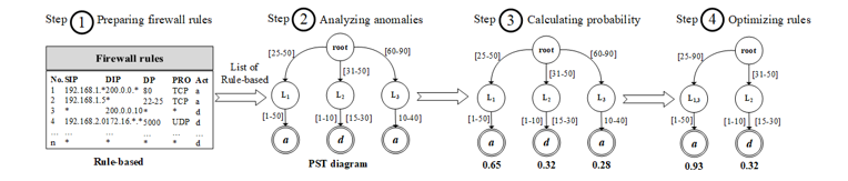Figure 2: Overview of the system design

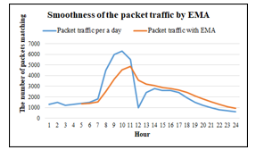Figure 3: Adjusting raw packets traffic to be more smooth by EMA

In the e_2 case: it refers to documents or pieces of paper used to confirm that such rules are approved to create them. In this paper, for example, the evidence for creating rules is divided into four levels: there is no evidence for approval, a firewall administrator is an approver, the head of the department is the approver, and approval is made by the owner of the organization. By dividing the weight of evidence according to the priority of the document approver: no evidence = 0, an administrator = 1, a head of the department = 2 and an owner of the organization = 3 respectively. If the weight of the document obtained is calculated by the Min-Max equation (8), the result will be the 〖e_2〗^’. Let the owner of the organization be approved to create the rule R_1, the result of the calculation is equal to:

〖e_2〗^’=(m- r_min)/(r_max-r_min )× t_max-t_min+t_min
=(3-0)/(3-0)×(1.0-0.0)+0.0=1.0

where m = 3, r_min = 0, r_max = 3, t_min = 0.0 and t_max is equal to 1.0.
In the e_3 case: similar in the case of evidence for creating rules, the expertise in creating rules is also divided into four levels: newbie admins, normal admins with sufficient expertise, professional admins and very expert administrators. The newbie admins mean those who have recently been assigned to configure the firewall system and have the least experience. When they have configured the firewall for a while, they will be more proficient, which should have at least 3 – 5 years of working hours, called normal admins. For those who have a lot of experience and training or firewall customization, with working hours of 5 – 10 years, they will be professional administrators. Finally, those who have received a lot of training and certificates about firewalls will be considered expert admins. From the statistics, those who are very skilled will be able to analyze and design firewall rules to minimize errors as well. In this paper, therefore, determines the weight of the following expertise e_3: newbie = 0, normal = 1, professional = 2 and very expertise administrator = 3. Let professional admins create the rule R_1, the result is calculated as.
〖e_3〗^’=(2-0)/(3-0)×(1.0-0.0)+0.0=0.66
In the e_4 case: the protocols communicating on the computer networks are always prioritized, such as video conferencing, and must be smooth throughout the meeting. On the other hand, sending electronic mail does not have an urgent need to be sent or received immediately. The protocol prioritization can be done depending on the policies of each organization. In this research, prioritization of the protocol is based on priorities from 3 GPP QoS Class Identification QCI categories [20] by IP Multimedia singling having the highest priority (1 = highest); Chat, FTP and P2P having the lowest priority (9 = lowest). From e_4 in Table 2, it is a teleconference application with a priority of 4.When processing in the form of probability using the Min-Max Scaling, the result is equal to:
〖e_4〗^’=(6-1)/(9-1)×(1.0-0.0)+0.0=0.625
Where m = 6 (Teleconference = 4), r_min = 1, r_max = 9, t_min = 0.0 and t_max is equal to 1.0. Notice that the priority of the protocols calculated must always reverse priorities, such as from 9 to 1 and from 1 to 9. For example, the priority of 4 is reversed to 6. Last, in Table 3, 4. represents examples of firewall rules consisting of all anomalies as previously mentioned, and these rules will be processed in the next step. Extra fields of each rule, when passing the data preparation process, it will produce the following results R_i→〖R_i〗^’.
Analyzing and Detecting Anomalies (Step 2)
In this phase, the rules from the 1st step are used to build a tree structure, called the Path Selection Tree (PST), to analyze the anomalies. The algorithm begins with the creation of the root node of PST. After that, field f_1 of the first rule is created as the first node on the tree, namely 〖SIP〗_1 as shown in Figure 4(a). In this node records source IP addresses of R_1 to be <R_1:[1, 100]>, where f_1 ∈ [1, 100]. The next node (〖DIP〗_1) stores the range of destination IP addresses (f_2) of R_1 ranging from 1 to 100. Next, it is the node that records source port ranges from 0 to 65535, called 〖SP〗_1. The next node as 〖DP〗_1, this node contains a group of destination ports f_4 between 80 and 85 (<R_1 : [80, 85]>). The final field f_5 of R_1 as 〖PRO〗_1 which keeps the range of TCP and UDP protocols. In the decision field, a bottom rectangular box in the tree, contains an acceptance decision (1) of R_1. At the end of the tree, it records what rules members of this path are like <R_1>.

Table 3: Examples of firewall rules (Ri)

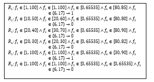
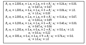
Table 4: Examples of extra fields (〖R_i〗^’)

In the next order, the second rule R_2 is imported into PST as illustrated in Figure 4(b). Firstly, f_1 of R_2 ⊂ f_1 of R_1, thus R_2 (f_1) uses the same route as R_1 (f_1) and also records <R_2:[10, 50]> into the 〖SIP〗_1 node. Likewise, R_2 (f_2) ⊂ R_1 (f_2), it is also recorded to the same node (〖DIP〗_1 = <R_1:[1, 100], R_2:[20, 60]>), and travels over the same route as R_1. Similar to R_2 (f_3), it is equal to R_1 (f_3), hence R_2 (f_3) is appended in the 〖SP〗_1 node to be <R_1, R_2:[0, 65536]>. In case of R_2 (f_4) and R_1 (f_4), R_2 (f_4) is a subset of R_1 (f_4), so the data of 〖DP〗_1 is updated as <R_1:[80, 85], R_2:[80, 80]> as well as 〖PRO〗_1 updated to <R_1, R_2:{6, 17}>. On the other hand, the decision of R_1 and R_2 are not the same, so the decision path must be separated from each other, where <R_1> = 1, <R_2> = 0. For inserting R_3 (Figure 4(c)) into PST, there is not much difference from inserting R_2, it is slightly different in the position of the protocol level in the tree. Since R_3(f_4) is a superset of R_1(f_4) and R_2(f_4), some destination ports of R_3(f_4) have to be separated into another node of the tree, namely 〖DP〗_2, which stores the destination ports ranging from 86 to 90 (R_3(f_4) – R_1(f_4)) like <R_3: [86, 90] >. Remaining destination ports are combined with 〖DIP〗_1 in the first path together with R_1 and R_2 as <R_1, R_3:[80, 85], R_2:[80, 80]>. The decision of R_3 is not allowed in both paths, where <R_3> = 0. Remaining firewall rules (R_4, R_5, R_6) will be executed like the previous rules (R_1, R_2, R_3). If all rules have been implemented successfully over PST, the results are shown in Figure 5.

In the process of checking the rule anomalies, the algorithm uses the information recorded on each node to detect anomalies by using the Cartesian product of all nodes separated from the protocol layer (〖PRO〗_i) and looking back from the bottom to the root as follows.

Group 1: path number 1 and 2 under the node 〖PRO〗_1

where CP is the Cartesian product. The results of each pair of the Cartesian product are calculated by equations (3) to (7) to find out what kind of anomalies they are. For example, in the equation (18) of group 1, (R_1,R_5) has the same decision (decision = 1), so it is executed by the equation (6). The result of the execution is a redundant anomaly. Next example, in equation (19), they consist of (R_2,R_3 ),(R_2,R_4 ),(R_2,R_6 ),(R_3,R_4 ),(R_3,R_6 ) and (R_4,R_6 ) by every pair of rules has the same decisions, thus all is executed by the equation (6) as same as the equation (18). Results of Cartesian product in the equation (20): (R_1,R_2 ),(R_1,R_3 ),(R_1,R_4 ),(R_1,R_6 ), (R_2,R_5 ),(R_3,R_5 ),(R_4,R_5 ) and (R_5,R_6 ), and every pair has different decisions, so they are executed by equations (3), (4) and (5) respectively. The calculated results: (R_2,R_3 ) = Redundancy and Semantics loss (Executed by equation (6)), (R_2,R_4 ) = Redundancy and Semantics loss (6), (R_2,R_6 ) = Redundancy and Semantics loss (6), (R_3,R_4 ) = Redundancy and Semantics loss (6), (R_3,R_6 ) = Redundancy and Semantics loss (6), (R_4,R_6 ) = Redundancy and Semantics loss (6), (R_1,R_2 ) = Shadowing (3), (R_1,R_3 ) = Correlation (4), (R_1,R_4 ) = Shadowing (3), (R_1,R_6 ) = Generalization (5), (R_2,R_5 ) = Generalization (5), (R_3,R_5 ) = Generalization (5), (R_4,R_5 ) = Generalization (5), (R_5,R_6 ) = Generalization (5). The results obtained from the calculations of group number 2 and 3 in equation 21 to 23: (R_3,R_6 ) = Redundancy and Semantics loss (Executed by equation (6)), (R_3,R_5 ) = Generalization (5), (R_5,R_6 ) = Generalization (5).
Losing the meaning of rules always occurs by redundant rules, thus all members in equations 18, 19 and 21 are possible to be the semantics loss as well.

Calculating Probability of Each Path of PST (Step 3)
The PST obtained from the previous steps is used to calculate the probability of each path in order to advise administrators to make decisions about optimizing firewall rules effectively, which has the following steps. Let R as a firewall rule, e as an attribute field of a rule, and S is a sample space, then the conditional probability of R given e is the equation (24) and shown in Figure 6.

 

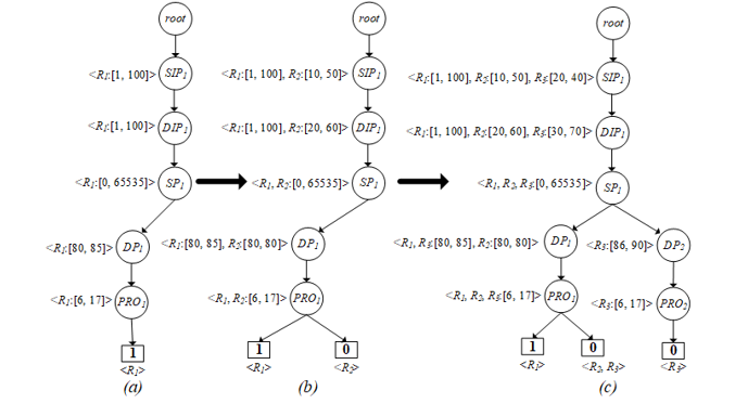Figure 4: Creating rule R_1 (a), R_2 (b) and R_3 (c) into PST

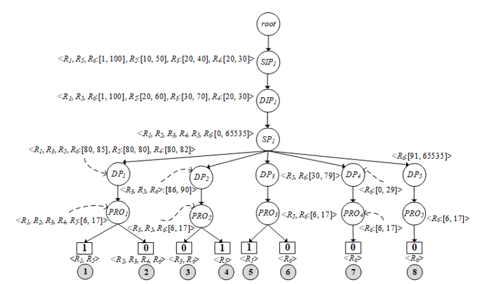Figure 5: Complete PST structure after compiling all rules

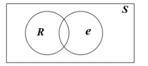Figure 6: Conditional probability of R given e in Venn diagram

 

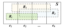Figure 7: Conditional probability of Ri given ek

According to Figure 7., given Ri as any rule, ek is any attribute (Extra field) of Ri:

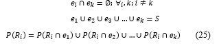
From the equation (24), P(R│e)=(P(R|e))/(P(e)), so P(R│e): P(e)P(R|e) or P(R)P(e|R). Since we already know the value of the P(e), then we choose P(R∩e) = P(e)P(R|e) and represent i and k into the equation as follows.

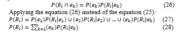
Given e_k is any property considering when giving P(R_i ) on the firewall. Finally, we can substitute this into Bayes’ rule (Equation 9) from above to obtain an alternative version of Bayes’ rule, which is used heavily in Bayesian inference:

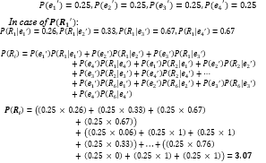
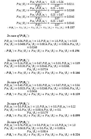
From examples of the property fields (Extra fields) in Table 4., there are four fields (〖e_1〗^’,〖e_2〗^’,〖e_3〗^’,〖e_4〗^’), where 〖e_1〗^’ = the frequency of packets matching against rules (FPM), 〖e_2〗^’ = evidence of creating rules (ECR), 〖e_3〗^’ = expertise of rules creator (ERC) and 〖e_4〗^’ = protocol priority (PRI). Assuming the weight of each feature is equal, so 〖e_1〗^’,〖e_2〗^’,〖e_3〗^’ and 〖e_4〗^’ are equal to 25% (0.25). Substituting various values in equations (28) and (29), the calculated results:

According to the weight of each rule property, admins can adjust the weight of each property as needed, such as 〖〖P(e〗_1〗^’)=35% (0.35),〖〖P(e〗_2〗^’)=15% (0.15),〖〖P(e〗_3〗^’)=25% (0.25) and 〖〖P(e〗_4〗^’)=25% (0.25) depending on each organization to give weight to their properties. After calculating all the probability values successfully, the algorithm inserts these probabilities to each path of PST as shown in Figure 8.

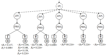Figure 8: Inserting probability of each Ri into PST

Optimizing Rule Anomalies (Last step)

Anomalies occurred over firewall rules have different solutions, for example, the redundant anomaly is solved by merging the rules together. However, this method may result in semantics loss instead. Other anomalies such as shadowing, correlation, and generalization, should not use the merging method because their decisions are different. Sometimes, administrators choose to resolve problems by switching rules, but they are not sure what will happen in the future. Therefore, this research uses the calculated probability in each rule to help administrators decide how to proceed with anomalies to achieve maximum efficiency and reasonableness. For example, the path number 1 of Figure 5., R_1 and R_5 are redundancy. If admins decide to combine the two rules together, the result is.

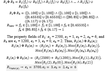
where 〖R_1〗_new as a new merged rule,  as a merging operator for the same decisions, Max is a function calculated the maximum value. In the same way as (R_2, R_3), (R_2, R_4),…, and (R_3, R_6), which are a redundant conflict, so they can solve the problem by combining rules like (R_1, R_5). The methods of resolving the remaining anomalies (Shadowing, Correlation, and Generalization) can be done in three ways: merging, swapping and removing rules. Nevertheless, admins must be highly skilled and aware of the consequences, almost all researchers do not recommend using these methods and often push the burden to the discretion of administrators instead. If the admins choose one of three methods, they can do by checking the probabilities of each rule. If the probability of any rule is the highest, it means that admins have the opportunity to resolve anomalies to be more effective. For example, (R_1, R_2) is the shadowing anomaly. If admins need to delete, merge or swap rules, they should give priority to R_2 rather than R_1 because R_2 is a higher probability (R_1 = 0.157, R_2 = 0.194) as shown in Figure 9.

 

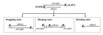Figure 9: Resolving shadowing by swapping, merging and deleting rules

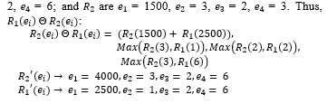
Updating property of R_1 and R_2 is not necessary in case of swapping and deleting rules, but in the case of merging, there are the following details.

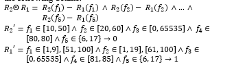
where  is a merging operator for different decisions. Although, R_2 (f_3 )-R_1 (f_3) and R_2 (f_5 )-R_1 (f_5) are equal to ∅. However, for this model, both are not equal to ∅ because they share the same path in the tree. The property fields of R_1: e_1 = 2500, e_2 = 1, e_3 = 2, e_4 = 6; and R_2 are e_1 = 1500, e_2 = 3, e_3 = 2, e_4 = 3.

Note that while updating each conflict rule each time, the PST structure will be changed, which means that the probability has to be recalculated whenever when resolving conflicts.

Implementation and Performance Evaluation

PST uses the k-ary tree structure (also known as m-ary or k-way tree) to develop, so the processing speed to build the tree is O(n), where n is the number of nodes of the given k-ary tree. The number of levels of the existing k-ary tree is L, the depth of the k-ary in the worst case is N-1, where N is the number of nodes in a tree. The k-ary tree can also be stored in breadth-first order as an implicit data structure in pointer-based, each node would have an internal array for storing pointers to each of its m children. So, the space complexity of k-ary tree structure is O(m ×n). Traversing the k-ary tree is very similar to binary tree traversal. Besides, the worst-case time complexity is O(〖log〗_m n). In practically, PST is developed on Intel Core i7 2.3 GHz, 8 GB RAM. The software developed includes Python language version 3.7 (64-bit), Graphviz [21] and NetworkX version 1.11 [22] running on Linux kernel (Version 4.4). The proposed model is illustrated in Figure 10.

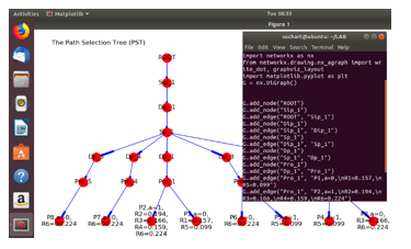Figure 10: The developed PST structure over Linux operating system

In this paper, we used x ̅ (Equation 13) to evaluate the satisfaction of the firewall administrators for resolving firewall rule anomalies of both traditional (No recommendation system) and our proposed firewall (Recommendation system with probability). In which of the confidence test consists of ten scenarios to resolve anomalies and the total number of testers (Firewall expert) is five as shown in Table 5.
Referring to Table 5, the average (x ̅) of the five administrators’ confidence for resolving ten scenarios of rule anomalies based on their skills for the traditional firewall is equal to 2.68; however, the average confidence of our proposed firewall which is a recommendation system based on probability is 4.16, which the confidence rate of the proposed firewall increased by 29.6% from the conventional firewall. In the case of evaluating reliability between raters, we apply Kappa statistics [19] in the equation (14) with the data from Table 5. The reliability value between the inter-raters of the conventional firewall is equal to 0.379, which means that the reliability is at a fair agreement as shown in Table 6. The reliability value between the assessors of the proposed firewall is equal to 0.510 (Moderate agreement), which means that the reliability increased from 37.9% to 51% significantly.
Table 5: Confidence tests to resolve anomalies of firewall rules

Firewall rule anomaly and resolving methods	The confidence of five admins for resolving rule anomalies
	Traditional firewalls (No the recommendation system) Admins judged by their experience					Our proposed firewall (Use the recommendation system) Admins judged by probability
	5	4	3	2	1	5	4	3	2	1
Shadowing
– Merging rules	1	1	2	1	0	0	0	1	2	2
– Swapping rules	1	1	2	0	1	0	0	1	3	1
– Deleting rules	0	2	2	1	0	0	0	2	2	1
Correlation
– Merging rules	1	2	2	0	0	0	0	1	2	2
– Swapping rules	0	2	2	1	0	0	0	1	2	2
Generalization
– Merging rules	1	2	2	0	0	0	0	2	1	2
– Swapping rules	1	1	2	1	0	0	0	1	2	2
– Deleting rules	0	1	2	1	1	0	0	1	2	2
Redundancy
– Merging rules	0	2	2	1	0	0	0	0	2	3
Semantics loss
– Merging rules	1	1	2	1	0	0	0	1	2	2

Remarks: the level of satisfaction is divided in to five levels: 5, 4, 3, 2, and 1; 5 is the highest confidence.
Table 6: Interpretation of the reliability between Inter-raters [19]

Kappa statistic value	Inter-rater reliability description
0	Agreement equivalent to chance
0.1 – 0.20	Alight agreement
0.21 – 0.40	Fair agreement
0.41 – 0.60	Moderate agreement
0.61 – 0.80	Substantial agreement
0.81 – 0.99	Near perfect agreement
1	Perfect agreement

Conclusion

Practically, fixing anomalies of firewall rules is quite complex, depending on the administrator’s perspective and experience. Correcting mistakes may lead to other anomalies. For example, when resolving the redundant anomaly, it may become the semantics loss of rules. In order to reduce the impact of errors and to resolve anomalies of administrators, this paper has designed and developed a system to assist in the decision-making of administrators by using probability together with four additional features of rules: frequency of matching between packets and rules, evidence of creating rules, expertise of rules creator and protocol priority. For each rule, the probability is calculated based on their features. If the probability of any rule is high, it indicates that the rule has a high priority. While rules in the firewall are conflicts, the rule that has a high probability value is always considered first. As a result of system testing, administrators can make more accurate decisions about conflict rules in the firewall. For the overall efficiency of the system, the time complexity of creating a system (PST) is equal to O(n), searching time over PST is O(〖log〗_m n) and the space complexity is O(m ×n). However, the system still has a limitation against the establishment of the tree structure. As resolving any anomaly of rules in each period, it needs to reconstruct the whole PST tree structure. For the evaluation of confidence for resolving firewall rule anomalies, the firewall that we have proposed on the basis of probability obtains a confidence value more than the traditional firewall by 29.6%, and the reliability between Inter-raters of proposed firewall is in the moderate agreement (0.51), which increased by 13.1% from the traditional firewall.

Acknowledgment

This research project was financially supported by Faculty of Informatics, Mahasarakham University 2020.

1. E. S. Al-Shaer and H. H. Hamed, “Modeling and management of firewall policies,” IEEE Transactions on Network and Service Management, 1(1), 2–10, April 2004. https://doi.org/10.1109/TNSM.2004.4623689
2. S. Khummanee, “The semantics loss tracker of firewall rules,” in IC2IT 2018 Recent Advances in Information and Communication Technology, 769, Jun. 2018, 220–231, 2018. https://doi.org/10.1007/978-3-319-93692-5_22
3. E. Al-Shaer, H. Hamed, R. Boutaba, and M. Hasan, “Conflict classification and analysis of distributed firewall policies,” IEEE Journal on Selected Areas in Communications, 23(10), 2069–2084, Oct 2005. https://doi.org/10.1109/JSAC.2005.854119
4. S. Khummanee, A. Khumseela, and S. Puangpronpitag, “Towards a new design of firewall: Anomaly elimination and fast verifying of firewall rules,” in The 2013 10th International Joint Conference on Computer Science and Software Engineering (JCSSE), May 2013, 93–98, 2013. https://doi.org/10.1109/JCSSE.2013.6567326
5. A. X. Liu, “Formal verification of firewall policies,” in 2008 IEEE International Conference on Communications, May 2008, 1494 – 1498, 2008. https://doi.org/10.1109/ICC.2008.289
6. M. Rezvani and R. Aryan, “Analyzing and resolving anomalies in firewall security policies based on propositional logic,” in 2009 IEEE 13th International Multitopic Conference, Dec 2009, 1–7, 2009. https://doi.org/10.1109/INMIC.2009.5383125
7. H. Hu, G. Ahn, and K. Kulkarni, “Detecting and resolving firewall policy anomalies,” IEEE Transactions on Dependable and Secure Computing, 9(3), 318–331, May 2012. https://doi.org/10.1109/TDSC.2012.20
8. S. R. Peter M. Mell, Karen A. Scarfone. (015) A complete guide to the common vulnerability scoring system version 2.0. [Online]. Available: https://www.nist.gov/publications/complete-guidecommon-vulnerability-scoring-system-version-20
9. A. Wool, “Architecting the lumeta firewall analyzer,” in SSYM’01 Proceedings of the 10th conference on USENIX Security Symposium, 10, Aug 2001, p. 7.
10. A. Mayer, A. Wool, and E. Ziskind, “Fang: a firewall analysis engine,” in Proceeding 2000 IEEE Symposium on Security and Privacy. S P 2000, May 2000, 177–187, 2000. https://doi.org/10.1109/SECPRI.2000.848455
11. A. Hari, S. Suri, and G. Parulkar, “Detecting and resolving packet filter conflicts,” in Proceedings IEEE INFOCOM 2000. Conference on Computer Communications. Nineteenth Annual Joint Conference of the IEEE Computer and Communications Societies (Cat. 00CH37064), 3, March 2000, 1203–1212 3, 2000. https://doi.org/10.1109/INFCOM.2000.832496
12. L. Zhang and M. Huang, “A firewall rules optimized model based on service-grouping,” in 2015 12th Web Information System and Application Conference (WISA), Sep. 2015, 142–146, 2015. https://doi.org/10.1109/WISA.2015.47
13. Lihua Yuan, Hao Chen, Jianning Mai, Chen-Nee Chuah, Zhendong Su, and P. Mohapatra, “Fireman: a toolkit for firewall modelling and analysis,” in 2006 IEEE Symposium on Security and Privacy (S P’06), May 2006, 15 –213, 2006. https://doi.org/10.1109/SP.2006.16
14. A. Saˆadaoui, N. B. Y. B. Souayeh, and A. Bouhoula, “Formal approach for managing firewall misconfigurations,” in 2014 IEEE Eighth International Conference on Research Challenges in Information Science (RCIS), May 2014, 1–10, 2014. https://doi.org/10.1109/RCIS.2014.6861044
15. W. Krombi, M. Erradi, and A. Khoumsi, “Automata-based approach to design and analyze security policies,” in 2014 Twelfth Annual International Conference on Privacy, Security and Trust, July 2014, 306–313, 2014. https://doi.org/10.1109/PST.2014.6890953
16. A. Saˆadaoui, N. B. Y. B. Souayeh, and A. Bouhoula, “Automated and optimized fdd-based method to fix firewall misconfigurations,” in 2015 IEEE 14th International Symposium on Network Computing and Applications, Sep. 2015, 63–67, 2015. https://doi.org/10.1109/NCA.2015.31
17. C. C. Aggarwal, Neural Networks and Deep Learning. Boca Raton, FL, USA: Springer, 2018.
18. D. Morris and M. Koning, Bayes’ Theorem Examples: A Visual Introduction for Beginners. 80 Strand, London, WC2R 0RL UK: Blue Windmill Media, 2016.
19. P. W. M. J. Kenneth J. Berry, Janis E. Johnston, The Measurement of Association: A Permutation Statistical Approach. Boca Raton, FL, USA: Springer, 2018.
20. CelPlan Technologies. Gpp qos class identification qci categories 2019. [Online]. Available: http://www.celplan.com
21. Graphviz. Graph visualization software 2019. [Online]. Available: https://www.graphviz.org
22. NetworkX. Software for complex networks, 2019. [Online]. Available: https://networkx.github.io

(Click Here)

(Click Here)