1. Introduction

In the management of a long electrical transmission line, fault location represents an important aspect, because it allows to reduce recovery times and increase network availability [1]. Currently, high voltage lines are protected by devices which allow to identify the fault position and put out of service the non-functioning part of the grid. For example, the distance protection employed on overhead transmission lines uses Intelligent Electronic Devices (IEDs) to estimate the impedance between the protection point and the failure point by measuring the line voltage and current [2]. In this way it is possible to obtain the distance from the fault, exploiting the correspondence between conductor impedance and length of the line section. In the last years new protection devices have been introduced, based on traveling wave detection; they allow to measure the impulsive signals generated by failures with greater precision [3]. However, these methods allow to locate the failure only once it has occurred [4].

 In this paper, an extension of a work originally presented at the International Conference on Soft Computing & Machine Intelligence (ISCMI 2019) [1], a system for monitoring the health status of the joints [1], [5] is presented. The system allows a preventive maintenance, so increasing the availability of the line. The joints (or junction regions) are the connection points between two different parts of the same phase conductor, and they represent one of the most stressed parts of overhead electrical lines [6], [7]. The proposed method exploits the equivalent lumped circuit of conductors and junction regions [8], [9]. In particular, the model of the elementary section of the network consists in the connection of the equivalent circuits of joint and conductor. The model of the whole line is obtained by the cascade connection of several elementary sections. The health status of the joint is obtained by measuring the network frequency response. To this aim it is necessary to establish a nominal working range for each electrical parameter of the line model. Any departure from this interval can be interpreted as a symptom of a possible fault. The deviation from the nominal condition is obtained through a comparison between the theoretical frequency response and measurements taken at several frequencies. The results of this comparison are traced back to the corresponding variation of the joint parameters. This operation is executed by a neural network able to classify the severity of the joint degradation. The selected neural network is a feedforward Multi-Layer network with Multi-Valued Neurons (MLMVN) whose training phase is carried out using the theoretical frequency response simulated on SapWin IV and MatLab^®. In this way it is possible to obtain a smart monitoring approach capable of classifying the measurements obtained through the PLC (Power Line Communication) systems [10]. This type of equipment is usually integrated on high and medium voltage networks to use the phase conductor as a channel for the transmission of information. Since the communication method is based on the modulation of the carrier wave, PLC systems can be used to generate signals with different frequencies obtaining measurements of the line transfer function [11].

The paper is organized as follows. Section 2 describes the model of conductors and joints. Section 3 is focused on the preliminary steps of the procedure, while section 4 is dedicated to the simulation procedure. Finally, Sections 5 and 6 report some specific application cases and conclusions, respectively.

2. Line Modelling

The main physical components of a line are junction regions and conductor stretches. The derivation of the equivalent circuits of these components represents the starting point for the line modelling. It is then necessary to establish the relationships between fault mechanisms and variation of electrical parameters. Only the joint degradation is considered in this paper and two different failure mechanisms are introduced: oxidation process and partial breakage of the joint structure. In this way it is possible to obtain three different intervals for the values of the electrical parameters, corresponding to the nominal situation, to the oxidation condition and to the presence of partial breaking [1].

2.1. Conductor modelling

In this paper an ACSR (Aluminum Conductor Steel Reinforced) with a diameter of 22.8 mm is used (Figure 1a). The equivalent model of the conductor (Figure 1b) contains four electrical elements and is called “canonical π-model”.

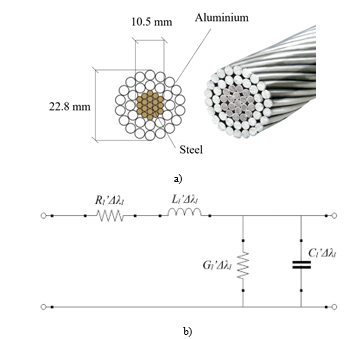Figure 1 – a) Physical structure of the conductor; b) Lumped circuit of the conductor.

It is commonly used to study wave propagation and power flow analysis [12], [13]. The term Δλ_l represents the conductor length, while the values of the parameters R_l’, L_l’, G_l’, C_l’ depend on the mechanical characteristics of the phase conductor; all these parameters are quantities per unit of length [14].

2.2 Joint modelling

Junction regions represent the connection points between two different parts of the same phase conductor, and they must guarantee the electrical continuity along the network [15], [16]. Bolted joints are used close to the pylons due to their high mechanical strength [17]. However, no available literature exists that describes their electrical behaviour; an acceptable alternative consists in modelling them with the better-known model of the solder joint, for which some information is available about its degradation mechanisms [18], [19]. The physical structure of the joint is shown in Figure 2a.

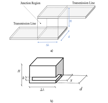Figure 2: a) Physical structure of the junction region; b) Braking parameters.

Δλ is the length of the junction region, d is its width and H its height. The characteristic parameters of the breaking mechanism are shown in Figure 2b where x represents the crack width and h is its height. The physical model and the equivalent lumped circuit of the joint are shown in Figure 3a and Figure 3b, respectively. In the equivalent circuit, the value of R_sj and L_sj in nominal conditions can be calculated by  and   respectively, while the capacitance value is nominally zero. If the frequency value used for the measurements exceeds the network frequency, it is necessary to consider the skin effect. For this reason, the penetration depth of the current (a frequency dependent parameter, calculated by ) is introduced and (1) is used to evaluate the resistance R_sj.

In oxidation conditions the resistance changes its value due to the increase of resistivity, while the partial breakage mechanism induces variations on the electrical parameters of the joint. In this work the consequentiality between oxidation mechanism and partial breakage process is assumed.

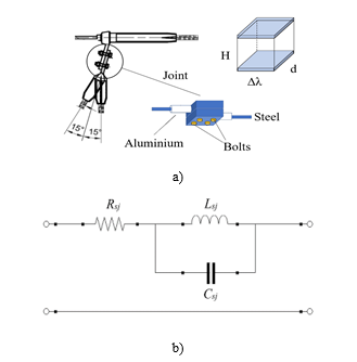Figure 3 – a) Physical model of the joint; b) Lumped circuit of the joint.

The formulas (2), (3) and (4) are obtained by introducing the typical breaking mechanism of solder joints and describing the variations of R_sj, L_sj and C_sj as functions of the crack width x and the crack height h [18]. Actually, only the R_sj and L_sj variations are considered, because the sensitivity of the C_sj variation is low.

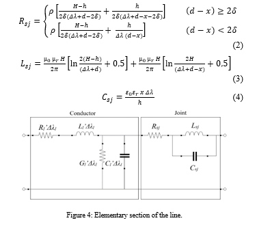  Figure 4: Elementary section of the line.

3. Problem outline

Once the equivalent lumped circuits of joint and conductor have been built, it is possible to describe the whole network by connecting in cascade the elementary line sections shown in Figure 4. Each line section between two pylons is represented by an elementary section and each joint model corresponds to the pylon position. A simplification is used in this case because there should be two joints and a short section of the conductor at the pylon. This is not a problem for the theoretical basis of the procedure presented in this paper, but it should be taken into account in practical applications [4, 1].

The next step of the procedure consists in the simulation of the model. This phase is needed for testability analysis, frequencies selection and neural network training, as shown in the following.

3.1. Testability analysis

It goes without saying that an a-priori knowledge of how many and which parameters are actually identifiable is quite useful in any fault diagnosis procedure, since it allows to correctly select the measurement test points. Testability analysis is exactly aimed at providing this kind of information [20, 21, 22]. It consists of two steps, testability evaluation and ambiguity groups identification. The testability gives the solvability degree of the fault diagnosis equations [23], i.e. it allows establishing the number of parameters whose value can be determined, starting from measurements taken on a given number of test points. The maximum possible value of testability is the number N of parameters present within the circuit under test. This maximum value is often not reached; this means that, in case of fault, there are parameters that are indistinguishable one to each other. In other words, it is possible to identify a set that contains the faulty component, but it is not possible to exactly identify the faulty one inside the group. The ambiguity groups are all those groups constituted by sets of indistinguishable parameters. The determination of the ambiguity groups gives information about which circuit parameters are identifiable.

In the procedure presented in this paper, testability analysis is a preliminary phase, aimed at discovering which and how many parameters of the line model are identifiable. This operation is executed starting from the network function, which acts as reference for the measurements, taken at selected frequencies. Consequently, it is necessary to simulate the line model in order to determine its network function.

3.2. Optimal frequency selection

As previously stated, the fault identification is the result of a comparison between the measurements at the test point and the nominal amplitude response, evaluated at the same frequencies. As shown in [24], measurement errors and manufacturing tolerances, which affect the result in a similar manner, depend on the choice of the frequencies. A proper selection allows minimizing the effect of these errors, increasing the probability to detect the fault. A method for carrying out this selection is presented in [24] and, in this work, it is used to obtain one test frequency. However, three octaves of the selected frequency are also used in the simulation procedure in order to make the system more robust and better train the complex neural network. It is worth pointing out that in [24] the use of more than one frequency has the scope to increase the number of equations, so that their number is at least as high as that of the unknown parameters. In the procedure presented in this paper there is no parameter identification, so there are no fault diagnosis equations to solve. Nevertheless, it is necessary to determine the network function of the line model in order to apply the procedure in [24], based on the network function derivatives.

3.3. Neural network training

The diagnosis method proposed in this paper uses neural networks, which do not require the derivation of fault equations. The analysis of the circuit model is however necessary for the training of the neural network, as it will be shown in the next section. The used intelligent classifier is a complex neural network, that presents excellent performances compared to other machine-learning techniques. It is based on a feedforward multilayer neural network with multi-valued neurons (MLMVN), characterized by a derivative free learning algorithm [25], an alternative algorithm based on the linear least square (LLS) methods [26] to reduce the high computational cost of the original backpropagation procedure, a soft margin method [27, 28] in order to make the network a good classifier. Further details will be given later in the application description.

4. Simulation Procedure

All the fundamental steps in the classification of the joint conditions are presented in this paragraph. First it is necessary to define the main characteristics of the network, the type of conductor and the physical size of the joints. Referring to the technical data sheets of the ACSR shown in Table 1, it is possible to obtain the value of the DC electrical resistance per unit of length R_l’ at ambient temperature (293K) and, consequently, the value of the resistivity . The conductor characteristics are extracted from [17], while the capacitance C_l’ and the inductance L_l’ are calculated assuming the transposition of the phase conductors. The formulas used in this case consider the number of conductors, their relative position and their diameter:

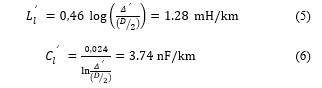
Table 1: Characteristic of the line conductor and bolted joint ASCR 22.8 Line Voltage [kV] Outer Diameter D [mm] Wire diameter (Al) [mm] Number of wires (Al) Wire Diameter (Steel) [mm] Number of wires (Steel) Rl’ [Ω/Km] 132 22.8 3.5 26 2.8 7 0.12 Bolted joint H [m] Δλ [m] d [m] Rsj [µΩ]   0.038     0.008   0.008   60

where Δ’ is the equivalent distance between the conductors (  ). The physical size of the joint and the nominal value of the DC electrical resistivity are extracted from [15] and shown in Table 1. The joint resistivity can be calculated through the equation .  In nominal conditions the inductance value L_sj is  and the capacitance C_sj is calculated by (4) assuming very low values for the breaking parameters (  and x ). In this way, it is possible to take into account the parasitic effects and maintain the same circuit topology for the nominal condition and the partial breaking condition. Therefore, the nominal value of the joint capacitance is .

4.1. Tolerance on the conductor electrical parameters

As previously stated, the conductors are assumed not faulty, hence they are set to their nominal values. Their resistance R_l’ depends on temperature and is subjected to the skin effect, on its time depending on the frequency f_m used for the measurements. The penetration depth of the current δ_l is given by the standard relation , where ρ_l and µ_l are respectively the resistivity of the conductor and the relative magnetic permeability. In order to obtain the correct value of the resistance, a parameter  is introduced, which is calculated as the ratio between the radius of the conductor and the penetration depth of the current. The electrical resistance of the conductor at ambient temperature (293K) can be obtained by multiplying R_l’ for a coefficient K so defined:

Then the final form of the electrical resistance is obtained by . As well known, the resistivity of a conductor changes its value with respect to the temperature. This means that there is a tolerance around the nominal resistance due to the conductor temperature. The definition of the resistance range is very important for verifying the performance of the monitoring system, since the neural network considers all the conductor components fixed at their nominal values, but the measurements of the frequency response change according to their real values. Therefore, the energy balance equation of transmission line is introduced [29, 30]:

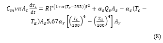where: T_c is the temperature of the conductor; T_α is the air temperature surrounding the conductor; C_m is the specific heat of the conductor materials; ν is the density of the conductor materials; A_t is the conductor section; A_s is the surface area receiving illumination with unit of length; A_c is the convection surface area; Ar is the radiation surface area per unit of length; α_c is the coefficient of convective heat; α_r is the radiation factor of the conductor materials; α_s is the sunshine absorption rate of the

Table 2: Characteristics of the conductor materials Cm [J/(kg K)] ν [kg/m3] At [m2] As [m2/m] Ar [m2/m] Ac [m2/m] αs   αc [W/(kg/m3)] αr   0.88 e-3 2.7 e3 π(D/2)2 π(D/2) πD πD 0.6 5.8 0.2

conductor; Q_s is the radiation intensity of the sun and sky. Within the equation there is the term R_l’ because it produces heat due to the Joule effect. It is necessary to observe that this is the value of the DC resistance considered equal to the resistance value at 50 Hz. The characteristics of the conductor material are extracted from [29] and reported in Table 2.

The expression of temperature variations as a function of time is obtained by solving the energy balance equation. In order to solve the equation, the initial conditions of the conductor, the radiation intensity Q_s and the air temperature T_α must be fixed. Typical values of Q_s and T_α, based on the measurements obtained in Italy in 2011, are used in this work. In the following, Q_smax represents the average of the maximum radiation levels for a specific month and T_αmax that of the maximum air temperatures. The average of the minimum temperature levels T_min is considered as the mean temperature in the night period and, for this reason, it is associated with a zero-radiation level. For simplification, the average values for each season are considered in Table 3. Once the load current has been fixed, the incidence of the environmental conditions on the resistance value can be obtained.

Table 3: Average values of solar radiation and temperature for each season

	Winter	Spring	Summer	Autumn
Qsmax  [W/m2]	392	753	750	357
Tαmax  [K]	281	295	301	284
Qsmin [W/m2]	0	0	0	0
Tαmin [K]	275	286	292	279

For example, if in summer the conductor temperature is calculated using (Q_smax;T_αmax), the maximum resistance error in the night period is about 16%. Considering the interval 0÷500 A for the load current and setting the environmental conditions, it is possible to obtain the incidence of the load on the resistance value. For example, in summer, the influence of the load current is about 7%. The worst situation for each season is presented in Table 4 and the errors are calculated assuming the maximum difference between the presumed and the real current. Similarly, the difference between the assumed and actual environmental conditions is maximized.

Table 4: Worst error for each season

Selected load current [A]	Real load current [A]	Error %
		Winter	Spring	Summer	Autumn
500	0	17.34	25.16	24.92	16.1

In this case the maximum error is made in spring and its percentage value is about 25,16%. By calculating the temperature with intermediate starting conditions between (Q_smax;T_αmax) and (Q_smin;T_αmin) and fixing the current at 250 A, it is possible to consider a 10÷12% variation range for the conductor resistance. Where (Q_smax;T_αmax)  and (Q_smin;T_αmin) are selected and real environmental condition respectively. The same variation range is extended to each electrical parameter of the conductor.

4.2. Circuit designing on SapWin IV

The simulator SapWin IV (Symbolic Analysis Program for Windows) [31, 32] is used for executing the circuit analysis and obtaining the symbolic network function of the model. The line admittance calculated at the starting point of the line is the network function. The first step of the fault procedure is the testability analysis, carried out by the program LINFTA [20] exploiting the SapWin IV simulation. Despite the fact that only the joint parameters are variable, all the electrical components are taken into account in the testability analysis. The circuits characterized by 2, 3, 4 and 5 elementary sections have been tested and the corresponding testability values are always maximum. The second step consists in the determination of the optimum set of frequencies. A program associated with the package SapWin IV performs this operation [24]. In this phase many circuit simulations are needed, at various different frequencies. The availability of the network function in symbolic form, as that provided by SAPWIN, is fundamental for keeping the processing times within reasonable limits. A single simulation is in fact sufficient, because, once the symbolic network function is available, it can be directly used to derive the response at all the desired frequencies. In the third step of the fault procedure the symbolic network function extracted from SapWin is processed on MatLab^® to obtain the training samples. Through a MatLab^® script, it is possible to set the conductor parameters at the numerical values and generate the training samples by varying the electrical components of each joint in its fault classes. Each conductor parameter is generated randomly in an interval of 10% around its nominal value, so taking into account the effects of environmental conditions and load current.

4.3. Fault classes and neural network setup

Three possible health states are considered for each junction region: nominal condition, structure oxidation and partial breakage. In order to obtain the correct classification of the working conditions by using the neural network, it is necessary to set the corresponding intervals for each electrical parameter. As mentioned above, the nominal value of the joint resistance is obtained from [17], while those of the inductance and capacitance have been calculated. Using the results presented in [17], it is also possible to define the resistance values in case of presence of the oxidation process (Table 5). These values represent the DC resistances of the joint in each operating condition and the

Table 5: Values of the joint resistance in the different oxidation conditions Nominal condition Low oxidation Medium oxidation High oxidation Ω m  Ω m  Ω m  Ω m

corresponding resistivities. The resistance values are given by (1) and we can note that the incidence of the skin effect decreases as the oxidation process increases. In fact, the oxidation process increases the resistivity of the material and, consequently, also increases the depth of the current penetration. Therefore, the skin effect is not relevant in the oxidation conditions, while it could introduce a false positive error in the nominal conditions.

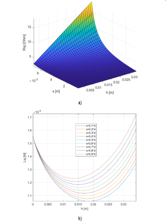Figure 5:  a) Resistance of the joint with respect to the crack height and crack width; b) Inductance of the joint with respect to the crack height and crack width

The skin effect can be also neglected in correspondence with the partial damage of the joint structure since the consequentiality between oxidation and breaking mechanism has been assumed. For this reason, only the second relation presented in (2) is used to describe the variation of the joint resistance with respect to the size of the crack (Figure 5a). In this case the resistivity  is used and  . The resistance of the joint  represents the upper limit in the oxidation conditions. The inductance variation with respect to the size of the crack is presented in Figure 5b and Figure 6a. According to the inductance value previously calculated, a tolerance of 0.2 µH is used to define the nominal conditions.

As shown in Figure 5b the value of L_sj leaves the interval of nominal conditions for h and x included between 10% and 65% of H and  respectively.

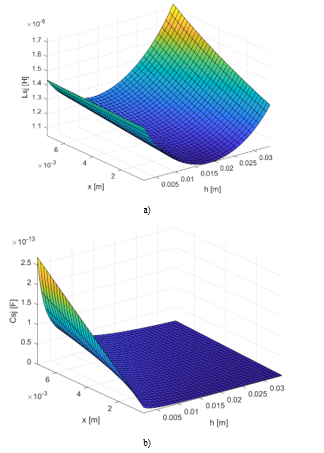Figure 6: a) Inductance of the joint with respect to the crack height and crack width; b) Capacitance of the joint with respect to the crack height and crack width

Since it is reasonable to consider equal percentage variations of x and h, since 65% of breakage represents a very high level of degradation, the interval chosen for the braking conditions is  neglecting the size of the crack for which the inductance returns in the nominal interval. Concerning the capacitance of the joint, its variation with respect to the size of the crack is shown in Figure 6b. Unfortunately, the sensitivity of the

Table 6: Fault classes Joint Parameters Nominal Condition Oxidation Condition Breaking Condition Rsj Lsj Csj

line frequency response with respect to the capacitance is low and, consequently, the value of C_sj is fixed to the nominal value.

Starting from these results the fault classes are defined. They are shown in Table 6. Once the equivalent lumped circuit has been obtained and the value of each electrical parameter has been defined, the complex neural network must be adapted in order to classify the health state of the joints.

The inputs of the neural network are the complex values corresponding to the network function at the selected frequencies. The network is characterized by two layers of neurons and two output neurons for each junction region (Figure 7).

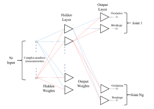Figure 7: Structure of the neural network

Each output neuron divides the complex plane in two different sectors (Figure 8) representing the nominal conditions and the presence of the failure mechanism.

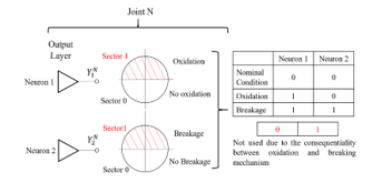Figure 8: Output combinations for each neuron

The first output neuron of each joint takes into account the oxidation process, while the second one considers the partial breaking mechanism. When the output level of both neurons is low (sector zero), the corresponding junction region is within the nominal conditions. If the first output is high (sector one) and the second one is low (sector zero), the combination represents the oxidation of the joint. If each output presents a high level (sector one), the corresponding junction region has partial damage. The last combination is not taken into consideration due to the hypothesis of the consequentiality between oxidation and partial breaking mechanism.

This paper uses a complex neural network implemented on MatLab^® version R2019b, but the whole code can also be used in previous versions of this software. Once the number of joints N_g has been set, there are  possible output combinations, since each junction region can be oxidized, broken or fully functional.

4.4. Neural network training and testing

The complex neural network used in this work, like other perceptron neural networks, has a good learning speed and allows to significantly reduce the computational cost by having a derivative free learning algorithm. Furthermore, the complex nature of this network is very suitable for dealing with electrical quantities and usually it is possible to obtain a better generalization capability in comparison with other neural networks and neuro-fuzzy networks. The learning rule is shown in (9):

where w_k+1 is the vector of the corrected weights, α_r is the learning constant, n is the number of the inputs, Z_k is the weighted sum, D is the desired output, Y is the actual output and  is the conjugate complex vector of the inputs.  Considering N_rs random samples for each combination, the matrix of the data sets presents  rows. Each row contains N_f magnitude measurements and N_f phase measurements of the same network function, with N_f number of test frequencies.

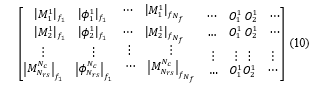Equation (10) shows the structure of the matrix containing the data sets. For example,  represents the second measure of magnitude corresponding to the first combination made at the frequency f₁,  represents the second measure of phase corresponding to the first combination made at the frequency f₁ and  is the second output of the first joint. Initially the weights of the neural network are randomly chosen and, subsequently, for each sample the error between the desired output and the actual one is calculated. The procedure shown in [26] is used to obtain the correction of the weights. This method uses a part of the total samples N_a, while the remaining part is used for the testing procedure. The backpropagation formulas calculate the error for each weight of the hidden layer and, then, the system shown in (11) is obtained.

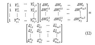
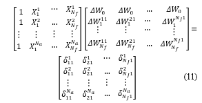For example,  is the first line input corresponding to the second sample,  represents the correction for the weight between the first input and the second neuron of the first layer, is the error on the second neuron of the first layer corresponding to the second sample. The values of the corrections are calculated through the Q-R decomposition and the same procedure is used for the output layer on the system shown in (12). The weight adjustment is repeated until the error satisfies the stopping criteria indicated in [27]. Therefore, there are two different stopping criteria: the first concerns the maximum number of classification errors that can be committed during the test phase and this means that the operator can set the maximum number of outputs that can be outside the desired sector . The second stopping criterion is chosen according to the rules of the soft margin technique and consists of a tolerance range on the distance between the value of each output and the bisector of the desired sector.

5. Results

Table 7: Dataset parameters for the simulation with three junction regions Ng Hidden Neurons Output Neurons Initial values of the weights Training samples Test samples Learning rate Classification rate 3 70 6 5 80% 20% 1 0.84074

All the fundamental steps in the classification of the joint conditions are presented in this paragraph to evaluate the performances of the proposed diagnostic method. The main objective of these simulations is to show that the system is able to identify the fault classes presented in Table 6, so confirming the validity of the presented prognostic approach for the predictive maintenance of high voltage electrical lines. A branch of electrical network containing three junction regions is the first configuration considered for the simulations. In this case, since the conductor length between two consecutive joints is 300 meters, the diagnostic system analyses approximately 900 meters of network. The analytical procedure shown in the paragraph 3.2 is used to obtain the optimal test frequency (f_m) and, starting from this value, also the next three octaves are considered to realize the dataset. This means that four signals are used to measure the line frequency response and, consequently, the network function magnitude and phase are calculated for each test frequency. The equivalent line admittance is used in this work. It corresponds to the ratio between the output current and the input voltage measured at the starting point of the network. From the theoretical point of view, the main steps to obtain the measurements are the equivalent circuit simulation on SapWin IV and the dataset generation on MatLab^®. The first step is the equivalent circuit simulation, which allows to obtain the symbolic formula of the line network function. For this reason, a cascade of three elementary sections (Figure 4) is realized on SapWin IV. The joint electrical parameters are kept symbolic, while the conductor components are set to their nominal values (as already said, taking into account the tolerances). Once the equivalent line admittance has been obtained, a specific MatLab^® code is used to generate the dataset. The main task of this code is to calculate the analytical formulas of magnitude and phase for each test frequency; subsequently the neural network inputs are calculated for each health state of the line by replacing the symbolic parameters with their numerical values. Since there are 3 junction regions in the first simulation (Ng = 3), 27 different combinations of the health state of the joints are obtained (  = 27) and, for each of them, 100 random samples (N_rs =100) are generated to complete the dataset. This means that each electrical parameter of the joints is randomly selected within one of the intervals shown in Table 6. The choice of 100 random samples is the result of some tests made to obtain a good compromise between the speed of processing and the representativeness of the dataset; it is not an optimized choice but it could, using specific techniques. Finally, the MatLab^® script uses the organization of the outputs shown in section 4 to associate the exact health state of the joints with each sample. Table 7 summarizes the situation for the first simulation. Finally, it is necessary to select the characteristics of the neural network, i.e. number of hidden neurons, initial values of the weights, learning rate, backpropagation procedure, computational method used for the weight adjustment. The last two are described in paragraph 4, while the fixed parameters of the neural network are selected through a heuristic approach. In particular, the number of hidden neurons is chosen through some tests to obtain good performances and a good generalization capability. A specific MatLab^® application is used to facilitate the selection, because it allows to obtain a very fast evaluation of the neural network performances by modifying the most important parameters.

The index used to evaluate neural network performances is called classification rate, and it is defined as the ratio between the number of correctly classified samples and the total number of samples used in the test phase. Indeed, only a percentage of the dataset is used for training the neural network, while the other samples are used to verify the correct functioning of the system. Table 8 presents the best neural network configuration for the first simulation and the corresponding value of the classification rate. The classification rate shown in Table 8 represents the global index to evaluate the performance of the diagnostic system and it is obtained by considering the classification errors made on 540 samples. This means that 2160 samples are used to modify the weight values during the training phase, while the remaining 540 samples are used to verify the results during the test phase.

Table 8: Complex neural network configuration for the simulation with three junction regions

Ng	Nrs	Nc	Nt	Dataset Input	Dataset Output	fm [kHz]
3	100	27	2700	8	6	35

It must be observed that each neuron has a specific classification rate greater than 0.84074 and this means that the performance of the system on a single junction region is much better than the global one. Table 9 shows the results obtained for each neuron and each junction region in the first configuration. Therefore, considering each joint separately, there is a probability range of 91÷95 % that the health state is correctly classified. It is not possible to establish a standard relationship between the classification rate for each pair of neurons and for the corresponding joint, because the number of errors for each junction region depends on the oxidation neuron, the rupture neuron or both.

Table 9: Results obtained for each joint and each neuron in the simulation with three junction regions

Fault class	Neuron	Classification Rate for each neuron	Joint	Classification Rate for each joint
Oxidation	1	0.9741	1	0.9470
Partial Breakage	2	0.9796
Oxidation	1	0.9685	2	0.9430
Partial Breakage	2	0.9977
Oxidation	1	0.9444	3	0.9130
Partial Breakage	2	0.9778

To get a more accurate evaluation of the system performance it is necessary to introduce the cross-validation method. In this case, the previously described training phase is repeated 5 times changing the learning data and the testing data. Therefore, the global classification rate is calculated on 2700 samples and represents the most reliable index. Cross-validation method is presented in Table 10 where the maximum and minimum classification rates represent the best and the worst result obtained at the end of each learning phase.

Table 10: Results obtained through the cross-validation method in the simulation with three junction regions

Fault class	Neuron	Joint	Maximum Classification Rate	Classification Rate
Oxidation	1	1	0.97037	0.9648
Partial Breakage	2		0.98889	0.9793
Oxidation	1	2	0.96481	0.9533
Partial Breakage	2		0.98333	0.9778
Oxidation	1	3	0.95000	0.9411
Partial Breakage	2		0.99259	0.9837
Global Classification Rate			0.8167

The same simulation procedure is used to evaluate the health state of a line with four junction regions. In this case 6480 samples are used to modify the weight values during the training phase, while the remaining 1620 samples are used to verify the results during the test phase. Table 11 summarizes the situation and shows the classification rate used to choose the neural network set up.

Table 11: Dataset and complex neural network set up for the simulation with four junction regions

Ng	Nrs	Nc	Nt
4	100	81	8100
Hidden Neurons	Output Neurons	Initial values of the weights	Training samples
190	8	5	80%
Dataset Input	Dataset Output	fm [kHz]	Test samples
8	8	80	20%
Classification rate
0.70247

Table 12: Results obtained through the cross-validation method in the simulation with four junction regions

Fault class	Neuron	Joint	Maximum Classification Rate	Classification Rate
Oxidation	1	1	0.97716	0.9700
Partial Breakage	2		0.98889	0.9830
Oxidation	1	2	0.93025	0.9188
Partial Breakage	2		0.98333	0.9757
Oxidation	1	3	0.94383	0.9367
Partial Breakage	2		0.98210	0.9781
Oxidation	1	4	0.91667	0.9046
Partial breakage	2		0.98333	0.9793
Global Classification Rate			0.6899

Also, in this case the cross-validation method is used to carry out the correct evaluation of the diagnostic system (Table 12). As mentioned above, by repeating the training phase 5 times, it is possible to evaluate all 8100 samples during the test phase. As shown in Table 12, the results obtained for each neuron are still excellent, while the global classification rate is lower than the first configuration. Obviously, increasing the number of the joints reduces the reliability of the complete system, which must be considered as a connection of four classifiers (one for each junction region). Therefore, if the main objective of the diagnostic system was to classify the exact combination of the health state of the joints, the system reliability is about 70%.

On the other hand, the working condition of each junction region can be classified with an accuracy level higher than 90%. This result is obtained considering each pair of output neurons separately (Table 13).

Table 13: Results obtained for each joint in the simulation with four junction regions

Joint	Classification Rate for each joint
1	0.9538
2	0.9006
3	0.9157
4	0.8854

The results presented in Table 13 can be used to compare the performance of the complex neural network with that of the other classifiers. Table 14 shows the comparison with one of the most used classifiers based on quadratic SVM (Support Vector Machine).

Table 14: Comparison between complex neural network and SVM classifier in the simulation with four junction regions

Joint	Classification for each joint with complex neural network	Classification rate for each joint with quadratic SVM
1	0.9538	0.9670
2	0.9006	0.8500
3	0.9157	0.8530
4	0.8854	0.8480

6. Conclusion

A diagnostic system based on a complex neural network has been presented and the procedure to obtain the state classification of the electrical joints has been verified through some different simulations. The results obtained for power lines characterized by three and four junction regions show that the system is able to identify the health state of each joint, with an accuracy level greater than 90%. The actual limit for the diagnostic method is represented by the line length, because the global classification rate obtained for a line with five joints is lower than the previous ones (Tables 15-16). Since the results obtained for the fifth junction region are not good, the system can be only used in a real application for small branches of the network. For this reason, future developments will concern the creation of a macroscopic method of locating failure mechanisms: the section of the non-functioning line could be localized through classification methods based on load flow measurements and after, the system presented in this work could be integrated to identify the junction region in the worst condition. In this way it would be possible to analyze a great variety of networks. Finally, a further development of the prognostic method could concern the analysis of the errors. The division between false positive and false negative errors is currently calculated, but no operation results from this. In the future, the method could be modified to minimize false negatives, which are the most dangerous errors for a diagnostic system

Table 15: Dataset and complex neural network configuration for the simulation with five junction regions

Ng	Nrs	Nc	Nt
5	100	243	24300
Hidden Neurons	Output Neurons	Initial values of the weights	Training samples
280	10	5	80%
Dataset Input	Dataset Output	fm [kHz]	Test samples
8	10	80	20%
Classification rate
0.098971

Table 15: Results obtained for each neuron in the case of five junction regions

Fault class	Neuron	Joint	Specific Classification Rate
Oxidation	1	1	0.9383
Partial Breakage	2		0.9885
Oxidation	1	2	0.7043
Partial Breakage	2		0.7648
Oxidation	1	3	0.7342
Partial Breakage	2		0.8438
Oxidation	1	4	0.7792
Partial breakage	2		0.9023
Oxidation	1	5	0.6780
Partial Breakage	2		0.6926

Conflict of Interest

The authors declare no conflict of interest.

Acknowledgment

Smart Energy Lab, University of Florence and Dept. of Information Engineering, University of Florence.

1. M. Bindi, F. Grasso, A. Luchetta, S. Manetti, M. C. Piccirilli, “Smart Monitoring and Fault Diagnosis of Joints in High Voltage Electrical Transmission Lines,” in 2019 6th International Conference on Soft Computing & Machine Intelligence (ISCMI), Johannesburg, South Africa, 40-44, 2019. doi: 10.1109/ISCMI47871.2019.9004307
2. Y. D. Liu, G. H. Sheng, Z. M. He, X. Y. Xu, X. C. Jiang, “Method of fault location based on the distributed traveling-wave detection device on overhead transmission line,” in 2011 IEEE Power Engineering and Automation Conference, Wuhan, 136-140, 2011. doi: 10.1109/PEAM.2011.6134925
3. X. Dong, S. Wang, S. Shi, “Research on characteristics of voltage fault traveling waves of transmission line”, in 2010 Modern Electric Power Systems, Wroclaw, 1-5, 2010. doi: 10.1109/MEPS16993.2010
4. L. Xun, L. Shungui, H. Ronghui, A. Jingwen, A. Yunzhu, C. Ping, X. Zhengxiang, “Study on accuracy traveling wave fault location method of overhead line — Cable hybrid line and its influencing factors,” in 2017 Chinese Automation Congress (CAC), Jinan, 4593-4597, 2017. doi: 10.1109/CAC.2017.8243590
5. M. Bindi, F. Grasso, A. Luchetta, S. Manetti, and M.C. Piccirilli “Modeling and diagnosis of joints in high voltage electrical transmission line”, in 2019 Proc. of Int. Conference on Energy, Electrical and Power Engineering (CEEPE 2019), IOP Conf. Series: Journal of Physics: Conf. Series 1304 (2019) 012006, 2019. doi:10.1088/1742-6596/1304/1/012006
6. R.K. Aggarwal, A.T. Johns, J.A.S.B. Jayasinghe, W Su, “An overview of the condition monitoring of overhead lines”, Electrical Power Systems Research 53, 15-12, 2000. https://doi.org/10.1016/S0378-7796(99)00037-1
7. C. Jinbing, W. Guogang, L. Huijun, “Mechanisms analysis and countermeasure of electrical contact overheating of overhead line,” in 2014 International Conference on Power System Technology, Chengdu, 1503-1508, 2014. doi: 10.1109/POWERCON.2014.6993786
8. G. Andersson, “Modelling and Analysis of Electric Power System”, PhD Thesis, ETH Zurich, 2008.
9. M. Davoudi, “Sensitivity Analysis of Power System State Estimation Regarding to Network Parameter Uncertainties”, PhD Thesis, Politecnico di Milano, 2012.
10. A. Cataliotti, V. Cosentino, D. D. Cara, G. Tinè, “Simulation of a power line communication system in medium and low voltage distribution networks” in 2011 IEEE International Workshop on Applied Measurements for Power Systems (AMPS), Aachen, 107-111, 2011. doi: 10.1109/AMPS.2011.6090429
11. A. Cataliotti, D. Di Cara, R. Fiorelli, G. Tine, “Power-Line Communication in Medium-Voltage System: Simulation Model and Onfield Experimental Tests,” IEEE Transactions on Power Delivery, 27(1), 62-69, 2012. doi: 10.1109/TPWRD.2011.2171009
12. J.S. Monteiro, W. L. A. Neves, D. Fernandes, B. A. Souza and A. B. Fernandes, “Computation of transmission line parameters for power flow studies,” in 2005 Canadian Conference on Electrical and Computer Engineering, Saskatoon, 607-610, 2005. doi: 10.1109/CCECE.2005.1557004
13. N.A. Jaffrey, S. Hettiwatte, “Corrosion detection in steel reinforced aluminium conductor cables,” in 2014 Australasian Universities Power Engineering Conference (AUPEC), Perth, WA, 1-6, 2014. doi: 10.1109/AUPEC.2014.6966630
14. G. M. Hashmi, M. Lehtonen, “Covered-Conductor Overhead Distribution Line Modeling and Experimental Verification for Determining its Line Characteristics,” in 2007 IEEE Power Engineering Society Conference and Exposition in Africa – PowerAfrica, Johannesburg, 1-7, 2007. doi: 10.1109/PESAFR.2007.4498072
15. F. Steier, “Tribologic analyses of a self-mated aluminium contact used for overhead transmission lines”, in 2017 Proc. of 6th Int. Conf. on Fracture Fatigue and Wear, IOP Conf. Series: Journal of Physics: Conf. Series 843 (2017) 012057, 2017. doi :10.1088/1742-6596/843/1/012057
16. Z. Liu, Y. Sun, “A solder joint crack — Characteristic impedance model based on transmission line theory,” in 2014 10th International Conference on Reliability, Maintainability and Safety (ICRMS), Guangzhou, 237-241, 2014. doi: 10.1109/ICRMS.2014.7107178
17. F. de Paulis, C. Olivieri, A. Orlandi, G. Giannuzzi, F. Bassi, C. Morandini, E. Fiorucci, G. Bucci, “Exploring Remote Monitoring of Degraded Compression and Bolted Joints in HV Power Transmission Lines,” IEEE Transactions on Power Delivery, 31(5), 2179-2187, 2016. doi: 10.1109/TPWRD.2016.2562579
18. M. H. Azarian, E. Lando, M. Pecht, “An analytical model of the RF impedance change due to solder joint cracking,” in 2011 IEEE 15th Workshop on Signal Propagation on Interconnects (SPI), Naples, 89-92, 2011. doi: 10.1109/SPI.2011.5898847
19. D. Achiriloaiei, S.V. Galatanu and I. Vetres, “Stress and strain determination occurring in contact area of 450/75 ACSR conductor”, in 2018 Proc. of 7th Int. Conf. on Advanced Materials and Structures AMS (Timisoara), IOP Conf. Series: Materials Science and Engineering 416 (2018) 012071, 2018. doi:10.1088/1757-899X/416/1/012071
20. G. Fontana, A. Luchetta, S. Manetti, M. C. Piccirilli, “A Fast Algorithm for Testability Analysis of Large Linear Time-Invariant Networks,” IEEE Transactions on Circuits and Systems I: Regular Papers, 64(6), 1564-1575, 2017. doi: 10.1109/TCSI.2016.2645079
21. G. Fontana, F. Grasso, A. Luchetta, S. Manetti, M. C. Piccirilli, A. Reatti, “A symbolic program for parameter identifiability analysis in systems modeled via equivalent linear time-invariant electrical circuits, with application to electromagnetic harvesters”, Int. J. of Numerical Modelling: Electronic Networks, Devices and Fields, 32, 2019. https://doi.org/10.1002/jnm.2251
22. G. Fontana, A. Luchetta, S. Manetti and M.C. Piccirilli, “An unconditionally sound algorithm for testability analysis in linear time invariant electrical networks” Int. J. Circ. Theor. Appl., 44, 1308-1340, 2016. doi: 10.1002/cta.2164
23. N. Sen and R. Saeks, “Fault diagnosis for linear systems via multifrequency measurements,” IEEE Transactions on Circuits and Systems, 26(7), 457-465, 1979. doi: 10.1109/TCS.1979.1084659
24. F. Grasso, A. Luchetta, S. Manetti, M. C. Piccirilli, “A Method for the Automatic Selection of Test Frequencies in Analog Fault Diagnosis,” IEEE Transactions on Instrumentation and Measurement, 56(6), 2322-2329, 2007. doi: 10.1109/TIM.2007.907947
25. I. Aizenberg, Complex-Valued Neural Networks with Multi-Valued Neurons. Berlin: Springer-Verlag Publishers, 2011.
26. I. Aizenberg, A. Luchetta, S. Manetti, “A modified learning algorithm for the multilayer neural network with multi-valued neurons based on the complex QR decomposition”, Soft Computing, 16, 563-575, 2012. doi: 10.1007/s00500-011-0755-7
27. I. Aizenberg, “MLMVN with Soft Margins Learning”, IEEE Transactions on Neural Networks and Learning Systems, 25, 1632-1644, 2014. doi: 10.1109/TNNLS.2014.2301802
28. E. Aizenberg, I. Aizenberg, “Batch linear least squares-based learning algorithm for MLMVN with soft margins,” in 2014 IEEE Symposium on Computational Intelligence and Data Mining (CIDM), Orlando, FL, 48-55, 2014. doi: 10.1109/CIDM.2014.7008147
29. Anjia Mao, Jing Wen and Shasha Luo, “A power system analysis model with consideration of environmental factors,” in 2010 5th International Conference on Critical Infrastructure (CRIS), Beijing, 1-5, 2010. doi: 10.1109/CRIS.2010.5617557
30. J. R. Santos, A. G. Exposito and F. P. Sanchez, “Assessment of conductor thermal models for grid studies,” IET Generation, Transmission & Distribution, 1(1), 155-161, 2007. doi: 10.1049/iet-gtd:20050472
31. F. Grasso, A. Luchetta, S. Manetti, M. C. Piccirilli and A. Reatti, “SapWin 4.0 – a new simulation program for electrical engineering education using symbolic analysis” Computer Application to Engineering Education, 24, 44–57, 2016. doi: 10.1002/cae.21671
32. www.sapwin.info Dept. of Information Engineering, University of Florence, Italy.

(Click Here)

(Click Here)